高效目标检测:YOLOV8 和 KerasCV
作者: Gitesh Chawda
创建日期 2023/06/26
最后修改日期 2023/06/26
描述: 使用 KerasCV 训练自定义 YOLOV8 目标检测模型。

简介
KerasCV 是 Keras 的一个用于计算机视觉任务的扩展。在此示例中,我们将了解如何使用 KerasCV 训练 YOLOV8 目标检测模型。
KerasCV 包含了流行的计算机视觉数据集(如 ImageNet、COCO 和 Pascal VOC)的预训练模型,可用于迁移学习。KerasCV 还提供了一系列可视化工具,用于检查模型学习到的中间表示,以及可视化目标检测和分割任务的结果。
如果您有兴趣了解如何使用 KerasCV 进行目标检测,我强烈建议您查看 lukewood 创建的指南。该资源可在 使用 KerasCV 进行目标检测 中找到,它提供了使用 KerasCV 构建目标检测模型所需的基本概念和技术的全面概述。
!pip install --upgrade git+https://github.com/keras-team/keras-cv -q
[33mWARNING: Running pip as the 'root' user can result in broken permissions and conflicting behaviour with the system package manager. It is recommended to use a virtual environment instead: https://pip.pypa.org.cn/warnings/venv[0m[33m
[0m
设置
import os
from tqdm.auto import tqdm
import xml.etree.ElementTree as ET

import tensorflow as tf
from tensorflow import keras

import keras_cv
from keras_cv import bounding_box
from keras_cv import visualization
/opt/conda/lib/python3.10/site-packages/tensorflow_io/python/ops/__init__.py:98: UserWarning: unable to load libtensorflow_io_plugins.so: unable to open file: libtensorflow_io_plugins.so, from paths: ['/opt/conda/lib/python3.10/site-packages/tensorflow_io/python/ops/libtensorflow_io_plugins.so']
caused by: ['/opt/conda/lib/python3.10/site-packages/tensorflow_io/python/ops/libtensorflow_io_plugins.so: undefined symbol: _ZN3tsl6StatusC1EN10tensorflow5error4CodeESt17basic_string_viewIcSt11char_traitsIcEENS_14SourceLocationE']
  warnings.warn(f"unable to load libtensorflow_io_plugins.so: {e}")
/opt/conda/lib/python3.10/site-packages/tensorflow_io/python/ops/__init__.py:104: UserWarning: file system plugins are not loaded: unable to open file: libtensorflow_io.so, from paths: ['/opt/conda/lib/python3.10/site-packages/tensorflow_io/python/ops/libtensorflow_io.so']
caused by: ['/opt/conda/lib/python3.10/site-packages/tensorflow_io/python/ops/libtensorflow_io.so: undefined symbol: _ZTVN10tensorflow13GcsFileSystemE']
  warnings.warn(f"file system plugins are not loaded: {e}")
加载数据
在本指南中,我们将使用从 roboflow 获取的自动驾驶汽车数据集。为了使数据集更易于管理,我从原始的 15,000 个数据样本的较大数据集中提取了一个子集。从这个子集中,我选择了 7,316 个样本用于模型训练。
为了简化当前任务并集中精力,我们将只处理较少的目标类别。具体来说,我们将考虑五个主要类别进行检测和分类:汽车、行人、交通信号灯、骑车人(biker)和卡车(truck)。这些类别代表了自动驾驶汽车场景中最常见和最重要的对象。
通过将数据集缩小到这些特定类别,我们可以专注于构建一个强大的目标检测模型,该模型能够准确地识别和分类这些重要对象。
TensorFlow Datasets 库提供了一种便捷的方式来下载和使用各种数据集,包括目标检测数据集。对于那些希望快速开始使用数据而无需手动下载和预处理数据的人来说,这是一个很好的选择。
您可以在 TensorFlow Datasets 中查看各种目标检测数据集。
然而,在此代码示例中,我们将演示如何使用 TensorFlow 的 tf.data 流水线从头开始加载数据集。这种方法提供了更大的灵活性,并允许您根据需要自定义预处理步骤。
加载 TensorFlow Datasets 库中不存在的自定义数据集是使用 tf.data 流水线的主要优势之一。这种方法允许您创建自定义数据预处理流水线,以满足您数据集的特定需求和要求。
超参数
SPLIT_RATIO = 0.2
BATCH_SIZE = 4
LEARNING_RATE = 0.001
EPOCH = 5
GLOBAL_CLIPNORM = 10.0
创建一个字典,将每个类名映射到一个唯一的数值标识符。此映射用于在目标检测任务的训练和推理过程中对类别标签进行编码和解码。
class_ids = [
    "car",
    "pedestrian",
    "trafficLight",
    "biker",
    "truck",
]
class_mapping = dict(zip(range(len(class_ids)), class_ids))

# Path to images and annotations
path_images = "/kaggle/input/dataset/data/images/"
path_annot = "/kaggle/input/dataset/data/annotations/"

# Get all XML file paths in path_annot and sort them
xml_files = sorted(
    [
        os.path.join(path_annot, file_name)
        for file_name in os.listdir(path_annot)
        if file_name.endswith(".xml")
    ]
)

# Get all JPEG image file paths in path_images and sort them
jpg_files = sorted(
    [
        os.path.join(path_images, file_name)
        for file_name in os.listdir(path_images)
        if file_name.endswith(".jpg")
    ]
)
下面的函数读取 XML 文件,找到图像名称和路径,然后遍历 XML 文件中的每个对象,提取每个对象的边界框坐标和类别标签。
该函数返回三个值:图像路径,一个边界框列表(每个边界框表示为包含四个浮点数的列表:xmin、ymin、xmax、ymax),以及一个与每个边界框对应的类别 ID 列表(表示为整数)。类别 ID 是通过使用名为 class_mapping 的字典将类别标签映射到整数值获得的。
def parse_annotation(xml_file):
    tree = ET.parse(xml_file)
    root = tree.getroot()

    image_name = root.find("filename").text
    image_path = os.path.join(path_images, image_name)

    boxes = []
    classes = []
    for obj in root.iter("object"):
        cls = obj.find("name").text
        classes.append(cls)

        bbox = obj.find("bndbox")
        xmin = float(bbox.find("xmin").text)
        ymin = float(bbox.find("ymin").text)
        xmax = float(bbox.find("xmax").text)
        ymax = float(bbox.find("ymax").text)
        boxes.append([xmin, ymin, xmax, ymax])

    class_ids = [
        list(class_mapping.keys())[list(class_mapping.values()).index(cls)]
        for cls in classes
    ]
    return image_path, boxes, class_ids


image_paths = []
bbox = []
classes = []
for xml_file in tqdm(xml_files):
    image_path, boxes, class_ids = parse_annotation(xml_file)
    image_paths.append(image_path)
    bbox.append(boxes)
    classes.append(class_ids)
0%| | 0/7316 [00:00<?, ?it/s]
在这里,我们使用 tf.ragged.constant 从 bbox 和 classes 列表创建稀疏张量。稀疏张量是一种可以处理沿一个或多个维度可变长度数据的张量类型。当处理具有可变长度序列的数据(如文本或时间序列数据)时,这非常有用。
classes = [
    [8, 8, 8, 8, 8],      # 5 classes
    [12, 14, 14, 14],     # 4 classes
    [1],                  # 1 class
    [7, 7],               # 2 classes
 ...]
bbox = [
    [[199.0, 19.0, 390.0, 401.0],
    [217.0, 15.0, 270.0, 157.0],
    [393.0, 18.0, 432.0, 162.0],
    [1.0, 15.0, 226.0, 276.0],
    [19.0, 95.0, 458.0, 443.0]],     #image 1 has 4 objects
    [[52.0, 117.0, 109.0, 177.0]],   #image 2 has 1 object
    [[88.0, 87.0, 235.0, 322.0],
    [113.0, 117.0, 218.0, 471.0]],   #image 3 has 2 objects
 ...]
在本例中,对于每张图像,bbox 和 classes 列表的长度都不同,具体取决于图像中的对象数量以及相应的边界框和类别。为了处理这种可变性,使用了稀疏张量而不是常规张量。
稍后,这些稀疏张量将通过 from_tensor_slices 方法用于创建 tf.data.Dataset。此方法通过沿第一个维度切片输入张量来从张量创建数据集。通过使用稀疏张量,数据集可以处理每张图像的可变长度数据,并为进一步处理提供灵活的输入流水线。
bbox = tf.ragged.constant(bbox)
classes = tf.ragged.constant(classes)
image_paths = tf.ragged.constant(image_paths)

data = tf.data.Dataset.from_tensor_slices((image_paths, classes, bbox))
将数据分割为训练数据和验证数据
# Determine the number of validation samples
num_val = int(len(xml_files) * SPLIT_RATIO)

# Split the dataset into train and validation sets
val_data = data.take(num_val)
train_data = data.skip(num_val)
让我们看看数据加载和边界框格式化,以开始工作。KerasCV 中的边界框具有预定的格式。为此,您必须将边界框捆绑到一个符合以下要求的字典中。
bounding_boxes = {
    # num_boxes may be a Ragged dimension
    'boxes': Tensor(shape=[batch, num_boxes, 4]),
    'classes': Tensor(shape=[batch, num_boxes])
}
该字典有两个键:'boxes' 和 'classes',每个键都映射到一个 TensorFlow 稀疏张量或张量对象。'boxes' 张量的形状为 [batch, num_boxes, 4],其中 batch 是批次中图像的数量,num_boxes 是任何图像中边界框的最大数量。4 代表定义边界框所需的四个值:xmin、ymin、xmax、ymax。
'classes' 张量的形状为 [batch, num_boxes],其中每个元素代表 'boxes' 张量中相应边界框的类别标签。num_boxes 维度可以是稀疏的,这意味着批次中图像之间的框数量可能不同。
最终字典应为
{"images": images, "bounding_boxes": bounding_boxes}
def load_image(image_path):
    image = tf.io.read_file(image_path)
    image = tf.image.decode_jpeg(image, channels=3)
    return image


def load_dataset(image_path, classes, bbox):
    # Read Image
    image = load_image(image_path)
    bounding_boxes = {
        "classes": tf.cast(classes, dtype=tf.float32),
        "boxes": bbox,
    }
    return {"images": tf.cast(image, tf.float32), "bounding_boxes": bounding_boxes}
这里我们创建一个图层,将图像调整为 640x640 像素,同时保持原始宽高比。图像的边界框以 xyxy 格式指定。如果需要,调整后的图像将用零填充以保持原始宽高比。
KerasCV 支持的边界框格式:1. CENTER_XYWH 2. XYWH 3. XYXY 4. REL_XYXY 5. REL_XYWH 6. YXYX 7. REL_YXYX
您可以在 文档 中详细了解 KerasCV 边界框格式。
此外,还可以执行任何两个对之间的格式转换。
boxes = keras_cv.bounding_box.convert_format(
        bounding_box,
        images=image,
        source="xyxy",  # Original Format
        target="xywh",  # Target Format (to which we want to convert)
    )
数据增强
构建目标检测流水线时,最具挑战性的任务之一是数据增强。它涉及对输入图像应用各种变换,以增加训练数据的多样性并提高模型的泛化能力。然而,在处理目标检测任务时,它变得更加复杂,因为这些变换需要了解底层的边界框并相应地更新它们。
KerasCV 为边界框增强提供了原生支持。KerasCV 提供了广泛的数据增强图层,专门用于处理边界框。这些图层会在图像变换时智能地调整边界框坐标,确保边界框保持准确并与增强后的图像对齐。
通过利用 KerasCV 的功能,开发人员可以方便地将对边界框友好的数据增强集成到他们的目标检测流水线中。通过在 tf.data 流水线中执行即时增强,该过程变得无缝且高效,从而实现更好的训练和更准确的目标检测结果。
augmenter = keras.Sequential(
    layers=[
        keras_cv.layers.RandomFlip(mode="horizontal", bounding_box_format="xyxy"),
        keras_cv.layers.RandomShear(
            x_factor=0.2, y_factor=0.2, bounding_box_format="xyxy"
        ),
        keras_cv.layers.JitteredResize(
            target_size=(640, 640), scale_factor=(0.75, 1.3), bounding_box_format="xyxy"
        ),
    ]
)
创建训练数据集
train_ds = train_data.map(load_dataset, num_parallel_calls=tf.data.AUTOTUNE)
train_ds = train_ds.shuffle(BATCH_SIZE * 4)
train_ds = train_ds.ragged_batch(BATCH_SIZE, drop_remainder=True)
train_ds = train_ds.map(augmenter, num_parallel_calls=tf.data.AUTOTUNE)
创建验证数据集
resizing = keras_cv.layers.JitteredResize(
    target_size=(640, 640),
    scale_factor=(0.75, 1.3),
    bounding_box_format="xyxy",
)

val_ds = val_data.map(load_dataset, num_parallel_calls=tf.data.AUTOTUNE)
val_ds = val_ds.shuffle(BATCH_SIZE * 4)
val_ds = val_ds.ragged_batch(BATCH_SIZE, drop_remainder=True)
val_ds = val_ds.map(resizing, num_parallel_calls=tf.data.AUTOTUNE)
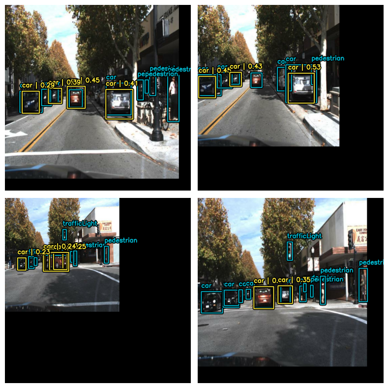
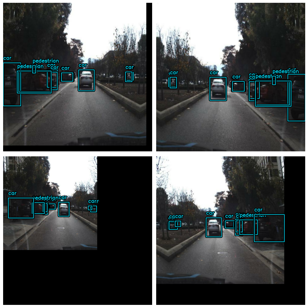
可视化
def visualize_dataset(inputs, value_range, rows, cols, bounding_box_format):
    inputs = next(iter(inputs.take(1)))
    images, bounding_boxes = inputs["images"], inputs["bounding_boxes"]
    visualization.plot_bounding_box_gallery(
        images,
        value_range=value_range,
        rows=rows,
        cols=cols,
        y_true=bounding_boxes,
        scale=5,
        font_scale=0.7,
        bounding_box_format=bounding_box_format,
        class_mapping=class_mapping,
    )


visualize_dataset(
    train_ds, bounding_box_format="xyxy", value_range=(0, 255), rows=2, cols=2
)

visualize_dataset(
    val_ds, bounding_box_format="xyxy", value_range=(0, 255), rows=2, cols=2
)
我们需要从预处理字典中提取输入,并准备好将它们输入模型。
def dict_to_tuple(inputs):
    return inputs["images"], inputs["bounding_boxes"]


train_ds = train_ds.map(dict_to_tuple, num_parallel_calls=tf.data.AUTOTUNE)
train_ds = train_ds.prefetch(tf.data.AUTOTUNE)

val_ds = val_ds.map(dict_to_tuple, num_parallel_calls=tf.data.AUTOTUNE)
val_ds = val_ds.prefetch(tf.data.AUTOTUNE)
创建模型
YOLOv8 是一款最先进的 YOLO 模型,用于各种计算机视觉任务,例如目标检测、图像分类和实例分割。YOLOv5 的创建者 Ultralytics 也开发了 YOLOv8,与前代产品相比,YOLOv8 在架构和开发者体验方面都进行了许多改进和更改。YOLOv8 是业内备受推崇的最新最先进模型。
下表比较了五种不同尺寸(以像素为单位)的 YOLOv8 模型(YOLOv8n、YOLOv8s、YOLOv8m、YOLOv8l 和 YOLOv8x)的性能指标。指标包括不同交并比 (IoU) 阈值下的平均精度 (mAP) 值(针对验证数据),在 CPU 上使用 ONNX 格式和 A100 TensorRT 的推理速度,参数数量,以及浮点运算次数 (FLOPs)(分别以百万和十亿为单位)。随着模型尺寸的增加,mAP、参数和 FLOPs 通常会增加,而速度则会降低。YOLOv8x 具有最高的 mAP、参数和 FLOPs,但推理速度最慢;而 YOLOv8n 的尺寸最小,推理速度最快,mAP、参数和 FLOPs 也最低。
| 模型 | 尺寸
(像素) | mAPval
50-95 | 速度
CPU ONNX
(毫秒) | 速度
A100 TensorRT
(毫秒) | 参数
(M) | FLOPs
(B) | | ------------------------------------------------------------------------------------ | --------------------- | -------------------- | ------------------------------ | ----------------------------------- | ------------------ | ----------------- | | YOLOv8n | 640 | 37.3 | 80.4 | 0.99 | 3.2 | 8.7 | | YOLOv8s | 640 | 44.9 | 128.4 | 1.20 | 11.2 | 28.6 | | YOLOv8m | 640 | 50.2 | 234.7 | 1.83 | 25.9 | 78.9 | | YOLOv8l | 640 | 52.9 | 375.2 | 2.39 | 43.7 | 165.2 | | YOLOv8x | 640 | 53.9 | 479.1 | 3.53 | 68.2 | 257.8 |
您可以在这个 RoboFlow 博客 中了解更多关于 YOLOV8 及其架构的信息。
首先,我们将创建用于我们 yolov8 检测器类的骨干实例。
KerasCV 中提供的 YOLOV8 骨干网络
- 无权重
1.   yolo_v8_xs_backbone
2.   yolo_v8_s_backbone
3.   yolo_v8_m_backbone
4.   yolo_v8_l_backbone
5.   yolo_v8_xl_backbone
- 带预训练的 coco 权重
backbone = keras_cv.models.YOLOV8Backbone.from_preset(
    "yolo_v8_s_backbone_coco"  # We will use yolov8 small backbone with coco weights
)
1.   yolo_v8_xs_backbone_coco
2.   yolo_v8_s_backbone_coco
2.   yolo_v8_m_backbone_coco
2.   yolo_v8_l_backbone_coco
2.   yolo_v8_xl_backbone_coco

Downloading data from https://storage.googleapis.com/keras-cv/models/yolov8/coco/yolov8_s_backbone.h5
20596968/20596968 [==============================] - 0s 0us/step
接下来,让我们使用 YOLOV8Detector 构建一个 YOLOV8 模型。YOLOV8Detector 接受一个特征提取器作为 backbone 参数,一个 num_classes 参数,用于根据 class_mapping 列表的大小指定要检测的对象类别数,一个 bounding_box_format 参数,用于告知模型数据集中 bbox 的格式,最后,特征金字塔网络 (FPN) 的深度由 fpn_depth 参数指定。
得益于 KerasCV,使用上述任何骨干网络构建 YOLOV8 非常简单。
yolo = keras_cv.models.YOLOV8Detector(
    num_classes=len(class_mapping),
    bounding_box_format="xyxy",
    backbone=backbone,
    fpn_depth=1,
)
编译模型
YOLOV8 使用的损失函数
-
分类损失:此损失函数计算预测类别概率与实际类别概率之间的差异。在此实例中,使用了
binary_crossentropy,这是二元分类问题的常用解决方案。我们使用二元交叉熵是因为每个识别出的对象要么被归类为属于某个特定对象类别(如人、汽车等),要么不属于。 -
框损失:
box_loss是用于衡量预测边界框与真实边界框之间差异的损失函数。在本例中,使用了完全交并比 (CIoU) 指标,该指标不仅测量预测边界框和真实边界框之间的重叠,还考虑了宽高比、中心距离和框大小的差异。这些损失函数共同通过最小化预测和真实类别概率以及边界框之间的差异来优化目标检测模型。
optimizer = tf.keras.optimizers.Adam(
    learning_rate=LEARNING_RATE,
    global_clipnorm=GLOBAL_CLIPNORM,
)

yolo.compile(
    optimizer=optimizer, classification_loss="binary_crossentropy", box_loss="ciou"
)
COCO 指标回调
我们将使用 KerasCV 的 BoxCOCOMetrics 来评估模型并计算 Map (平均精度) 分数、召回率和精确率。我们还会保存模型,当 mAP 分数提高时。
class EvaluateCOCOMetricsCallback(keras.callbacks.Callback):
    def __init__(self, data, save_path):
        super().__init__()
        self.data = data
        self.metrics = keras_cv.metrics.BoxCOCOMetrics(
            bounding_box_format="xyxy",
            evaluate_freq=1e9,
        )

        self.save_path = save_path
        self.best_map = -1.0

    def on_epoch_end(self, epoch, logs):
        self.metrics.reset_state()
        for batch in self.data:
            images, y_true = batch[0], batch[1]
            y_pred = self.model.predict(images, verbose=0)
            self.metrics.update_state(y_true, y_pred)

        metrics = self.metrics.result(force=True)
        logs.update(metrics)

        current_map = metrics["MaP"]
        if current_map > self.best_map:
            self.best_map = current_map
            self.model.save(self.save_path)  # Save the model when mAP improves

        return logs
训练模型
yolo.fit(
    train_ds,
    validation_data=val_ds,
    epochs=3,
    callbacks=[EvaluateCOCOMetricsCallback(val_ds, "model.h5")],
)
Epoch 1/3
1463/1463 [==============================] - 633s 390ms/step - loss: 10.1535 - box_loss: 2.5659 - class_loss: 7.5876 - val_loss: 3.9852 - val_box_loss: 3.1973 - val_class_loss: 0.7879 - MaP: 0.0095 - MaP@[IoU=50]: 0.0193 - MaP@[IoU=75]: 0.0074 - MaP@[area=small]: 0.0021 - MaP@[area=medium]: 0.0164 - MaP@[area=large]: 0.0010 - Recall@[max_detections=1]: 0.0096 - Recall@[max_detections=10]: 0.0160 - Recall@[max_detections=100]: 0.0160 - Recall@[area=small]: 0.0034 - Recall@[area=medium]: 0.0283 - Recall@[area=large]: 0.0010
Epoch 2/3
1463/1463 [==============================] - 554s 378ms/step - loss: 2.6961 - box_loss: 2.2861 - class_loss: 0.4100 - val_loss: 3.8292 - val_box_loss: 3.0052 - val_class_loss: 0.8240 - MaP: 0.0077 - MaP@[IoU=50]: 0.0197 - MaP@[IoU=75]: 0.0043 - MaP@[area=small]: 0.0075 - MaP@[area=medium]: 0.0126 - MaP@[area=large]: 0.0050 - Recall@[max_detections=1]: 0.0088 - Recall@[max_detections=10]: 0.0154 - Recall@[max_detections=100]: 0.0154 - Recall@[area=small]: 0.0075 - Recall@[area=medium]: 0.0191 - Recall@[area=large]: 0.0280
Epoch 3/3
1463/1463 [==============================] - 558s 381ms/step - loss: 2.5930 - box_loss: 2.2018 - class_loss: 0.3912 - val_loss: 3.4796 - val_box_loss: 2.8472 - val_class_loss: 0.6323 - MaP: 0.0145 - MaP@[IoU=50]: 0.0398 - MaP@[IoU=75]: 0.0072 - MaP@[area=small]: 0.0077 - MaP@[area=medium]: 0.0227 - MaP@[area=large]: 0.0079 - Recall@[max_detections=1]: 0.0120 - Recall@[max_detections=10]: 0.0257 - Recall@[max_detections=100]: 0.0258 - Recall@[area=small]: 0.0093 - Recall@[area=medium]: 0.0396 - Recall@[area=large]: 0.0226

<keras.callbacks.History at 0x7f3e01ca6d70>
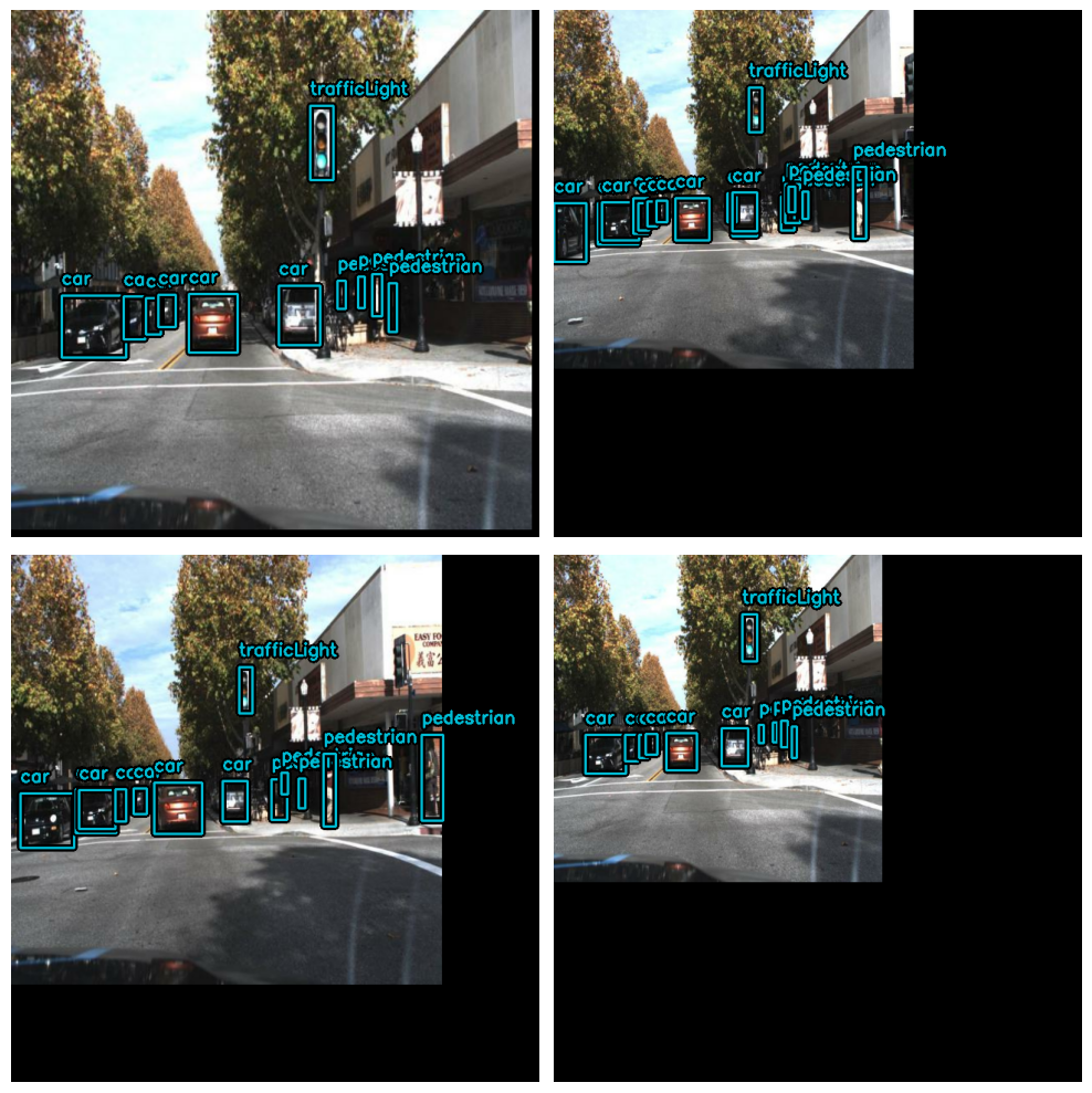
可视化预测
def visualize_detections(model, dataset, bounding_box_format):
    images, y_true = next(iter(dataset.take(1)))
    y_pred = model.predict(images)
    y_pred = bounding_box.to_ragged(y_pred)
    visualization.plot_bounding_box_gallery(
        images,
        value_range=(0, 255),
        bounding_box_format=bounding_box_format,
        y_true=y_true,
        y_pred=y_pred,
        scale=4,
        rows=2,
        cols=2,
        show=True,
        font_scale=0.7,
        class_mapping=class_mapping,
    )


visualize_detections(yolo, dataset=val_ds, bounding_box_format="xyxy")
1/1 [==============================] - 0s 115ms/step