无
使用卷积 LSTM 进行下一帧视频预测
作者: Amogh Joshi
创建日期 2021/06/02
最后修改日期 2023/11/10
描述: 如何构建和训练用于下一帧视频预测的卷积 LSTM 模型。

简介
卷积 LSTM 架构通过在 LSTM 层中引入卷积循环单元,将时间序列处理与计算机视觉结合起来。在本示例中,我们将探索卷积 LSTM 模型在下一帧预测中的应用,即根据一系列过去的帧预测后续视频帧的过程。
设置
import numpy as np
import matplotlib.pyplot as plt

import keras
from keras import layers

import io
import imageio
from IPython.display import Image, display
from ipywidgets import widgets, Layout, HBox
数据集构建
在本示例中,我们将使用 Moving MNIST 数据集。
我们将下载数据集,然后构建并预处理训练集和验证集。
对于下一帧预测,我们的模型将使用前一帧(我们称之为 f_n)来预测新一帧(称之为 f_(n + 1))。为了使模型能够进行这些预测,我们需要处理数据,使其具有“移位”的输入和输出,其中输入数据是帧 x_n,用于预测帧 y_(n + 1)。
# Download and load the dataset.
fpath = keras.utils.get_file(
    "moving_mnist.npy",
    "http://www.cs.toronto.edu/~nitish/unsupervised_video/mnist_test_seq.npy",
)
dataset = np.load(fpath)

# Swap the axes representing the number of frames and number of data samples.
dataset = np.swapaxes(dataset, 0, 1)
# We'll pick out 1000 of the 10000 total examples and use those.
dataset = dataset[:1000, ...]
# Add a channel dimension since the images are grayscale.
dataset = np.expand_dims(dataset, axis=-1)

# Split into train and validation sets using indexing to optimize memory.
indexes = np.arange(dataset.shape[0])
np.random.shuffle(indexes)
train_index = indexes[: int(0.9 * dataset.shape[0])]
val_index = indexes[int(0.9 * dataset.shape[0]) :]
train_dataset = dataset[train_index]
val_dataset = dataset[val_index]

# Normalize the data to the 0-1 range.
train_dataset = train_dataset / 255
val_dataset = val_dataset / 255


# We'll define a helper function to shift the frames, where
# `x` is frames 0 to n - 1, and `y` is frames 1 to n.
def create_shifted_frames(data):
    x = data[:, 0 : data.shape[1] - 1, :, :]
    y = data[:, 1 : data.shape[1], :, :]
    return x, y


# Apply the processing function to the datasets.
x_train, y_train = create_shifted_frames(train_dataset)
x_val, y_val = create_shifted_frames(val_dataset)

# Inspect the dataset.
print("Training Dataset Shapes: " + str(x_train.shape) + ", " + str(y_train.shape))
print("Validation Dataset Shapes: " + str(x_val.shape) + ", " + str(y_val.shape))
Downloading data from http://www.cs.toronto.edu/~nitish/unsupervised_video/mnist_test_seq.npy
 819200096/819200096 ━━━━━━━━━━━━━━━━━━━━ 116s 0us/step
Training Dataset Shapes: (900, 19, 64, 64, 1), (900, 19, 64, 64, 1)
Validation Dataset Shapes: (100, 19, 64, 64, 1), (100, 19, 64, 64, 1)
数据可视化
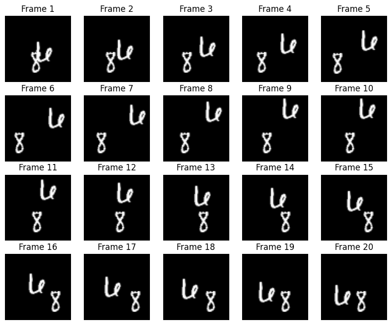
我们的数据由帧序列组成,每个帧序列都用于预测后续帧。让我们来看一些这些连续的帧。
# Construct a figure on which we will visualize the images.
fig, axes = plt.subplots(4, 5, figsize=(10, 8))

# Plot each of the sequential images for one random data example.
data_choice = np.random.choice(range(len(train_dataset)), size=1)[0]
for idx, ax in enumerate(axes.flat):
    ax.imshow(np.squeeze(train_dataset[data_choice][idx]), cmap="gray")
    ax.set_title(f"Frame {idx + 1}")
    ax.axis("off")

# Print information and display the figure.
print(f"Displaying frames for example {data_choice}.")
plt.show()
Displaying frames for example 95.
模型构建
为了构建卷积 LSTM 模型,我们将使用 ConvLSTM2D 层,该层将接受形状为 (batch_size, num_frames, width, height, channels) 的输入,并返回相同形状的预测视频。
# Construct the input layer with no definite frame size.
inp = layers.Input(shape=(None, *x_train.shape[2:]))

# We will construct 3 `ConvLSTM2D` layers with batch normalization,
# followed by a `Conv3D` layer for the spatiotemporal outputs.
x = layers.ConvLSTM2D(
    filters=64,
    kernel_size=(5, 5),
    padding="same",
    return_sequences=True,
    activation="relu",
)(inp)
x = layers.BatchNormalization()(x)
x = layers.ConvLSTM2D(
    filters=64,
    kernel_size=(3, 3),
    padding="same",
    return_sequences=True,
    activation="relu",
)(x)
x = layers.BatchNormalization()(x)
x = layers.ConvLSTM2D(
    filters=64,
    kernel_size=(1, 1),
    padding="same",
    return_sequences=True,
    activation="relu",
)(x)
x = layers.Conv3D(
    filters=1, kernel_size=(3, 3, 3), activation="sigmoid", padding="same"
)(x)

# Next, we will build the complete model and compile it.
model = keras.models.Model(inp, x)
model.compile(
    loss=keras.losses.binary_crossentropy,
    optimizer=keras.optimizers.Adam(),
)
模型训练
构建好模型和数据后,我们现在可以训练模型了。
# Define some callbacks to improve training.
early_stopping = keras.callbacks.EarlyStopping(monitor="val_loss", patience=10)
reduce_lr = keras.callbacks.ReduceLROnPlateau(monitor="val_loss", patience=5)

# Define modifiable training hyperparameters.
epochs = 20
batch_size = 5

# Fit the model to the training data.
model.fit(
    x_train,
    y_train,
    batch_size=batch_size,
    epochs=epochs,
    validation_data=(x_val, y_val),
    callbacks=[early_stopping, reduce_lr],
)
Epoch 1/20
 180/180 ━━━━━━━━━━━━━━━━━━━━ 50s 226ms/step - loss: 0.1510 - val_loss: 0.2966 - learning_rate: 0.0010
Epoch 2/20
 180/180 ━━━━━━━━━━━━━━━━━━━━ 40s 219ms/step - loss: 0.0287 - val_loss: 0.1766 - learning_rate: 0.0010
Epoch 3/20
 180/180 ━━━━━━━━━━━━━━━━━━━━ 40s 219ms/step - loss: 0.0269 - val_loss: 0.0661 - learning_rate: 0.0010
Epoch 4/20
 180/180 ━━━━━━━━━━━━━━━━━━━━ 40s 219ms/step - loss: 0.0264 - val_loss: 0.0279 - learning_rate: 0.0010
Epoch 5/20
 180/180 ━━━━━━━━━━━━━━━━━━━━ 40s 219ms/step - loss: 0.0258 - val_loss: 0.0254 - learning_rate: 0.0010
Epoch 6/20
 180/180 ━━━━━━━━━━━━━━━━━━━━ 40s 219ms/step - loss: 0.0256 - val_loss: 0.0253 - learning_rate: 0.0010
Epoch 7/20
 180/180 ━━━━━━━━━━━━━━━━━━━━ 40s 219ms/step - loss: 0.0251 - val_loss: 0.0248 - learning_rate: 0.0010
Epoch 8/20
 180/180 ━━━━━━━━━━━━━━━━━━━━ 40s 219ms/step - loss: 0.0251 - val_loss: 0.0251 - learning_rate: 0.0010
Epoch 9/20
 180/180 ━━━━━━━━━━━━━━━━━━━━ 40s 219ms/step - loss: 0.0247 - val_loss: 0.0243 - learning_rate: 0.0010
Epoch 10/20
 180/180 ━━━━━━━━━━━━━━━━━━━━ 40s 219ms/step - loss: 0.0246 - val_loss: 0.0246 - learning_rate: 0.0010
Epoch 11/20
 180/180 ━━━━━━━━━━━━━━━━━━━━ 40s 219ms/step - loss: 0.0245 - val_loss: 0.0247 - learning_rate: 0.0010
Epoch 12/20
 180/180 ━━━━━━━━━━━━━━━━━━━━ 40s 219ms/step - loss: 0.0241 - val_loss: 0.0243 - learning_rate: 0.0010
Epoch 13/20
 180/180 ━━━━━━━━━━━━━━━━━━━━ 40s 219ms/step - loss: 0.0244 - val_loss: 0.0245 - learning_rate: 0.0010
Epoch 14/20
 180/180 ━━━━━━━━━━━━━━━━━━━━ 40s 219ms/step - loss: 0.0241 - val_loss: 0.0241 - learning_rate: 0.0010
Epoch 15/20
 180/180 ━━━━━━━━━━━━━━━━━━━━ 40s 219ms/step - loss: 0.0243 - val_loss: 0.0241 - learning_rate: 0.0010
Epoch 16/20
 180/180 ━━━━━━━━━━━━━━━━━━━━ 40s 219ms/step - loss: 0.0242 - val_loss: 0.0242 - learning_rate: 0.0010
Epoch 17/20
 180/180 ━━━━━━━━━━━━━━━━━━━━ 40s 219ms/step - loss: 0.0240 - val_loss: 0.0240 - learning_rate: 0.0010
Epoch 18/20
 180/180 ━━━━━━━━━━━━━━━━━━━━ 40s 219ms/step - loss: 0.0240 - val_loss: 0.0243 - learning_rate: 0.0010
Epoch 19/20
 180/180 ━━━━━━━━━━━━━━━━━━━━ 40s 219ms/step - loss: 0.0240 - val_loss: 0.0244 - learning_rate: 0.0010
Epoch 20/20
 180/180 ━━━━━━━━━━━━━━━━━━━━ 40s 219ms/step - loss: 0.0237 - val_loss: 0.0238 - learning_rate: 1.0000e-04

<keras.src.callbacks.history.History at 0x7ff294f9c340>
帧预测可视化
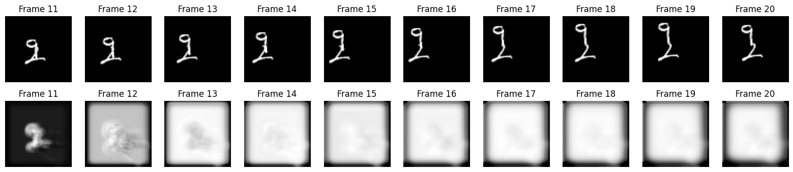
现在模型已经构建并训练完成,我们可以基于新视频生成一些示例帧预测。
我们将从验证集中随机选择一个示例,然后从中选取前十帧。在此基础上,我们可以让模型预测 10 个新帧,然后将其与真实帧预测进行比较。
# Select a random example from the validation dataset.
example = val_dataset[np.random.choice(range(len(val_dataset)), size=1)[0]]

# Pick the first/last ten frames from the example.
frames = example[:10, ...]
original_frames = example[10:, ...]

# Predict a new set of 10 frames.
for _ in range(10):
    # Extract the model's prediction and post-process it.
    new_prediction = model.predict(np.expand_dims(frames, axis=0))
    new_prediction = np.squeeze(new_prediction, axis=0)
    predicted_frame = np.expand_dims(new_prediction[-1, ...], axis=0)

    # Extend the set of prediction frames.
    frames = np.concatenate((frames, predicted_frame), axis=0)

# Construct a figure for the original and new frames.
fig, axes = plt.subplots(2, 10, figsize=(20, 4))

# Plot the original frames.
for idx, ax in enumerate(axes[0]):
    ax.imshow(np.squeeze(original_frames[idx]), cmap="gray")
    ax.set_title(f"Frame {idx + 11}")
    ax.axis("off")

# Plot the new frames.
new_frames = frames[10:, ...]
for idx, ax in enumerate(axes[1]):
    ax.imshow(np.squeeze(new_frames[idx]), cmap="gray")
    ax.set_title(f"Frame {idx + 11}")
    ax.axis("off")

# Display the figure.
plt.show()
 1/1 ━━━━━━━━━━━━━━━━━━━━ 2s 2s/step
 1/1 ━━━━━━━━━━━━━━━━━━━━ 1s 800ms/step
 1/1 ━━━━━━━━━━━━━━━━━━━━ 1s 805ms/step
 1/1 ━━━━━━━━━━━━━━━━━━━━ 1s 790ms/step
 1/1 ━━━━━━━━━━━━━━━━━━━━ 1s 821ms/step
 1/1 ━━━━━━━━━━━━━━━━━━━━ 1s 824ms/step
 1/1 ━━━━━━━━━━━━━━━━━━━━ 1s 928ms/step
 1/1 ━━━━━━━━━━━━━━━━━━━━ 1s 813ms/step
 1/1 ━━━━━━━━━━━━━━━━━━━━ 1s 810ms/step
 1/1 ━━━━━━━━━━━━━━━━━━━━ 1s 814ms/step
预测视频
最后,我们将从验证集中选取一些示例,并用它们制作一些 GIF,以查看模型的预测视频。
您可以使用托管在 Hugging Face Hub 上的训练模型,并在 Hugging Face Spaces 上试用演示。
# Select a few random examples from the dataset.
examples = val_dataset[np.random.choice(range(len(val_dataset)), size=5)]

# Iterate over the examples and predict the frames.
predicted_videos = []
for example in examples:
    # Pick the first/last ten frames from the example.
    frames = example[:10, ...]
    original_frames = example[10:, ...]
    new_predictions = np.zeros(shape=(10, *frames[0].shape))

    # Predict a new set of 10 frames.
    for i in range(10):
        # Extract the model's prediction and post-process it.
        frames = example[: 10 + i + 1, ...]
        new_prediction = model.predict(np.expand_dims(frames, axis=0))
        new_prediction = np.squeeze(new_prediction, axis=0)
        predicted_frame = np.expand_dims(new_prediction[-1, ...], axis=0)

        # Extend the set of prediction frames.
        new_predictions[i] = predicted_frame

    # Create and save GIFs for each of the ground truth/prediction images.
    for frame_set in [original_frames, new_predictions]:
        # Construct a GIF from the selected video frames.
        current_frames = np.squeeze(frame_set)
        current_frames = current_frames[..., np.newaxis] * np.ones(3)
        current_frames = (current_frames * 255).astype(np.uint8)
        current_frames = list(current_frames)

        # Construct a GIF from the frames.
        with io.BytesIO() as gif:
            imageio.mimsave(gif, current_frames, "GIF", duration=200)
            predicted_videos.append(gif.getvalue())

# Display the videos.
print(" Truth\tPrediction")
for i in range(0, len(predicted_videos), 2):
    # Construct and display an `HBox` with the ground truth and prediction.
    box = HBox(
        [
            widgets.Image(value=predicted_videos[i]),
            widgets.Image(value=predicted_videos[i + 1]),
        ]
    )
    display(box)
 1/1 ━━━━━━━━━━━━━━━━━━━━ 0s 6ms/step
 1/1 ━━━━━━━━━━━━━━━━━━━━ 0s 5ms/step
 1/1 ━━━━━━━━━━━━━━━━━━━━ 0s 5ms/step
 1/1 ━━━━━━━━━━━━━━━━━━━━ 0s 5ms/step
 1/1 ━━━━━━━━━━━━━━━━━━━━ 0s 6ms/step
 1/1 ━━━━━━━━━━━━━━━━━━━━ 0s 6ms/step
 1/1 ━━━━━━━━━━━━━━━━━━━━ 0s 8ms/step
 1/1 ━━━━━━━━━━━━━━━━━━━━ 0s 7ms/step
 1/1 ━━━━━━━━━━━━━━━━━━━━ 0s 7ms/step
 1/1 ━━━━━━━━━━━━━━━━━━━━ 1s 790ms/step
 1/1 ━━━━━━━━━━━━━━━━━━━━ 0s 5ms/step
 1/1 ━━━━━━━━━━━━━━━━━━━━ 0s 5ms/step
 1/1 ━━━━━━━━━━━━━━━━━━━━ 0s 5ms/step
 1/1 ━━━━━━━━━━━━━━━━━━━━ 0s 5ms/step
 1/1 ━━━━━━━━━━━━━━━━━━━━ 0s 6ms/step
 1/1 ━━━━━━━━━━━━━━━━━━━━ 0s 6ms/step
 1/1 ━━━━━━━━━━━━━━━━━━━━ 0s 7ms/step
 1/1 ━━━━━━━━━━━━━━━━━━━━ 0s 7ms/step
 1/1 ━━━━━━━━━━━━━━━━━━━━ 0s 8ms/step
 1/1 ━━━━━━━━━━━━━━━━━━━━ 0s 8ms/step
 1/1 ━━━━━━━━━━━━━━━━━━━━ 0s 6ms/step
 1/1 ━━━━━━━━━━━━━━━━━━━━ 0s 6ms/step
 1/1 ━━━━━━━━━━━━━━━━━━━━ 0s 5ms/step
 1/1 ━━━━━━━━━━━━━━━━━━━━ 0s 6ms/step
 1/1 ━━━━━━━━━━━━━━━━━━━━ 0s 6ms/step
 1/1 ━━━━━━━━━━━━━━━━━━━━ 0s 6ms/step
 1/1 ━━━━━━━━━━━━━━━━━━━━ 0s 7ms/step
 1/1 ━━━━━━━━━━━━━━━━━━━━ 0s 7ms/step
 1/1 ━━━━━━━━━━━━━━━━━━━━ 0s 7ms/step
 1/1 ━━━━━━━━━━━━━━━━━━━━ 0s 8ms/step
 1/1 ━━━━━━━━━━━━━━━━━━━━ 0s 6ms/step
 1/1 ━━━━━━━━━━━━━━━━━━━━ 0s 5ms/step
 1/1 ━━━━━━━━━━━━━━━━━━━━ 0s 6ms/step
 1/1 ━━━━━━━━━━━━━━━━━━━━ 0s 6ms/step
 1/1 ━━━━━━━━━━━━━━━━━━━━ 0s 7ms/step
 1/1 ━━━━━━━━━━━━━━━━━━━━ 0s 8ms/step
 1/1 ━━━━━━━━━━━━━━━━━━━━ 0s 6ms/step
 1/1 ━━━━━━━━━━━━━━━━━━━━ 0s 7ms/step
 1/1 ━━━━━━━━━━━━━━━━━━━━ 0s 7ms/step
 1/1 ━━━━━━━━━━━━━━━━━━━━ 0s 9ms/step
 1/1 ━━━━━━━━━━━━━━━━━━━━ 0s 5ms/step
 1/1 ━━━━━━━━━━━━━━━━━━━━ 0s 5ms/step
 1/1 ━━━━━━━━━━━━━━━━━━━━ 0s 5ms/step
 1/1 ━━━━━━━━━━━━━━━━━━━━ 0s 5ms/step
 1/1 ━━━━━━━━━━━━━━━━━━━━ 0s 6ms/step
 1/1 ━━━━━━━━━━━━━━━━━━━━ 0s 6ms/step
 1/1 ━━━━━━━━━━━━━━━━━━━━ 0s 6ms/step
 1/1 ━━━━━━━━━━━━━━━━━━━━ 0s 7ms/step
 1/1 ━━━━━━━━━━━━━━━━━━━━ 0s 8ms/step
 1/1 ━━━━━━━━━━━━━━━━━━━━ 0s 10ms/step
 Truth  Prediction

HBox(children=(Image(value=b'GIF89a@\x00@\x00\x87\x00\x00\xff\xff\xff\xfe\xfe\xfe\xfd\xfd\xfd\xfc\xfc\xfc\xf8\…

HBox(children=(Image(value=b'GIF89a@\x00@\x00\x86\x00\x00\xff\xff\xff\xfd\xfd\xfd\xfc\xfc\xfc\xfb\xfb\xfb\xf4\…

HBox(children=(Image(value=b'GIF89a@\x00@\x00\x86\x00\x00\xff\xff\xff\xfe\xfe\xfe\xfd\xfd\xfd\xfc\xfc\xfc\xfb\…

HBox(children=(Image(value=b'GIF89a@\x00@\x00\x86\x00\x00\xff\xff\xff\xfe\xfe\xfe\xfd\xfd\xfd\xfc\xfc\xfc\xfb\…

HBox(children=(Image(value=b'GIF89a@\x00@\x00\x86\x00\x00\xff\xff\xff\xfd\xfd\xfd\xfc\xfc\xfc\xf9\xf9\xf9\xf7\…