► 代码示例 / 计算机视觉 / 计算机视觉中的学习图像缩放

计算机视觉中的学习图像缩放

作者： Sayak Paul
创建日期 2021/04/30
最后修改 2023/12/18
描述： 如何针对给定分辨率最佳地学习图像表示。

ⓘ 此示例使用 Keras 3

人们普遍认为，如果我们将视觉模型限制为像人类一样感知事物，其性能可以得到提升。例如，在这项工作中，Geirhos 等人表明，在 ImageNet-1k 数据集上预训练的视觉模型偏向于纹理，而人类主要使用形状描述符来形成共同感知。但是，这种观点是否总是适用，特别是在提升视觉模型性能方面？

事实证明并非总是如此。在训练视觉模型时，通常会将图像大小调整到较低维度（例如 (224 x 224), (299 x 299) 等），以便进行小批量学习并适应计算限制。我们通常使用诸如双线性插值之类的图像缩放方法进行此步骤，并且缩放后的图像对人眼而言不会损失太多感知特性。在《学习为计算机视觉任务调整图像大小》一文中，Talebi 等人表明，如果我们尝试优化图像对视觉模型而非人眼的感知质量，它们的性能可以进一步提升。他们研究了以下问题：

对于给定的图像分辨率和模型，如何最佳地调整给定图像的大小？

如论文所示，这个想法有助于持续提升常见视觉模型（在 ImageNet-1k 上预训练）的性能，例如 DenseNet-121、ResNet-50、MobileNetV2 和 EfficientNets。在本示例中，我们将实现论文中提出的可学习图像缩放模块，并使用 DenseNet-121 架构在 Cats and Dogs 数据集上进行演示。

设置

import os

os.environ["KERAS_BACKEND"] = "tensorflow"
import keras
from keras import ops
from keras import layers
import tensorflow as tf

import tensorflow_datasets as tfds

tfds.disable_progress_bar()

import matplotlib.pyplot as plt
import numpy as np

定义超参数

为了方便小批量学习，我们需要在给定批次中为图像设置固定的形状。这就是为什么需要进行初始缩放。我们首先将所有图像缩放为 (300 x 300) 形状，然后学习它们在 (150 x 150) 分辨率下的最佳表示。

INP_SIZE = (300, 300)
TARGET_SIZE = (150, 150)
INTERPOLATION = "bilinear"

AUTO = tf.data.AUTOTUNE
BATCH_SIZE = 64
EPOCHS = 5

在本示例中，我们将使用双线性插值，但可学习图像缩放模块不依赖于任何特定的插值方法。我们也可以使用其他方法，例如双三次插值。

加载和准备数据集

在本示例中，我们将只使用总训练数据集的 40%。

train_ds, validation_ds = tfds.load(
    "cats_vs_dogs",
    # Reserve 10% for validation
    split=["train[:40%]", "train[40%:50%]"],
    as_supervised=True,
)


def preprocess_dataset(image, label):
    image = ops.image.resize(image, (INP_SIZE[0], INP_SIZE[1]))
    label = ops.one_hot(label, num_classes=2)
    return (image, label)


train_ds = (
    train_ds.shuffle(BATCH_SIZE * 100)
    .map(preprocess_dataset, num_parallel_calls=AUTO)
    .batch(BATCH_SIZE)
    .prefetch(AUTO)
)
validation_ds = (
    validation_ds.map(preprocess_dataset, num_parallel_calls=AUTO)
    .batch(BATCH_SIZE)
    .prefetch(AUTO)
)

定义可学习缩放工具

下图（来源：《学习为计算机视觉任务调整图像大小》）展示了可学习缩放模块的结构：

def conv_block(x, filters, kernel_size, strides, activation=layers.LeakyReLU(0.2)):
    x = layers.Conv2D(filters, kernel_size, strides, padding="same", use_bias=False)(x)
    x = layers.BatchNormalization()(x)
    if activation:
        x = activation(x)
    return x


def res_block(x):
    inputs = x
    x = conv_block(x, 16, 3, 1)
    x = conv_block(x, 16, 3, 1, activation=None)
    return layers.Add()([inputs, x])

    # Note: user can change num_res_blocks to >1 also if needed


def get_learnable_resizer(filters=16, num_res_blocks=1, interpolation=INTERPOLATION):
    inputs = layers.Input(shape=[None, None, 3])

    # First, perform naive resizing.
    naive_resize = layers.Resizing(*TARGET_SIZE, interpolation=interpolation)(inputs)

    # First convolution block without batch normalization.
    x = layers.Conv2D(filters=filters, kernel_size=7, strides=1, padding="same")(inputs)
    x = layers.LeakyReLU(0.2)(x)

    # Second convolution block with batch normalization.
    x = layers.Conv2D(filters=filters, kernel_size=1, strides=1, padding="same")(x)
    x = layers.LeakyReLU(0.2)(x)
    x = layers.BatchNormalization()(x)

    # Intermediate resizing as a bottleneck.
    bottleneck = layers.Resizing(*TARGET_SIZE, interpolation=interpolation)(x)

    # Residual passes.
    # First res_block will get bottleneck output as input
    x = res_block(bottleneck)
    # Remaining res_blocks will get previous res_block output as input
    for _ in range(num_res_blocks - 1):
        x = res_block(x)

    # Projection.
    x = layers.Conv2D(
        filters=filters, kernel_size=3, strides=1, padding="same", use_bias=False
    )(x)
    x = layers.BatchNormalization()(x)

    # Skip connection.
    x = layers.Add()([bottleneck, x])

    # Final resized image.
    x = layers.Conv2D(filters=3, kernel_size=7, strides=1, padding="same")(x)
    final_resize = layers.Add()([naive_resize, x])

    return keras.Model(inputs, final_resize, name="learnable_resizer")


learnable_resizer = get_learnable_resizer()

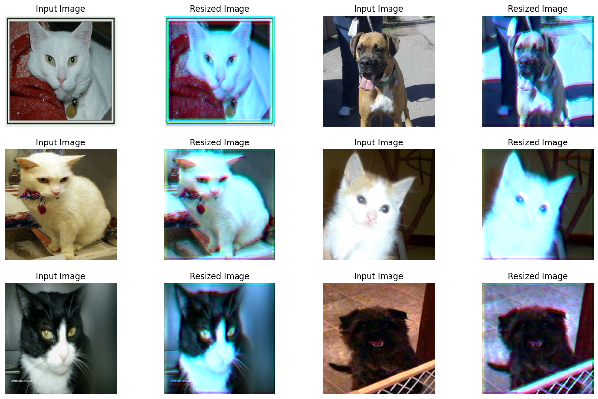
可视化可学习缩放模块的输出

在这里，我们可视化图像经过缩放器随机权重处理后的样子。

sample_images, _ = next(iter(train_ds))


plt.figure(figsize=(16, 10))
for i, image in enumerate(sample_images[:6]):
    image = image / 255

    ax = plt.subplot(3, 4, 2 * i + 1)
    plt.title("Input Image")
    plt.imshow(image.numpy().squeeze())
    plt.axis("off")

    ax = plt.subplot(3, 4, 2 * i + 2)
    resized_image = learnable_resizer(image[None, ...])
    plt.title("Resized Image")
    plt.imshow(resized_image.numpy().squeeze())
    plt.axis("off")

Corrupt JPEG data: 65 extraneous bytes before marker 0xd9
WARNING:matplotlib.image:Clipping input data to the valid range for imshow with RGB data ([0..1] for floats or [0..255] for integers).
WARNING:matplotlib.image:Clipping input data to the valid range for imshow with RGB data ([0..1] for floats or [0..255] for integers).
WARNING:matplotlib.image:Clipping input data to the valid range for imshow with RGB data ([0..1] for floats or [0..255] for integers).
WARNING:matplotlib.image:Clipping input data to the valid range for imshow with RGB data ([0..1] for floats or [0..255] for integers).
WARNING:matplotlib.image:Clipping input data to the valid range for imshow with RGB data ([0..1] for floats or [0..255] for integers).
WARNING:matplotlib.image:Clipping input data to the valid range for imshow with RGB data ([0..1] for floats or [0..255] for integers).

png

模型构建工具

def get_model():
    backbone = keras.applications.DenseNet121(
        weights=None,
        include_top=True,
        classes=2,
        input_shape=((TARGET_SIZE[0], TARGET_SIZE[1], 3)),
    )
    backbone.trainable = True

    inputs = layers.Input((INP_SIZE[0], INP_SIZE[1], 3))
    x = layers.Rescaling(scale=1.0 / 255)(inputs)
    x = learnable_resizer(x)
    outputs = backbone(x)

    return keras.Model(inputs, outputs)

可学习图像缩放模块的结构可以灵活地与不同的视觉模型集成。

使用可学习缩放器编译和训练我们的模型

model = get_model()
model.compile(
    loss=keras.losses.CategoricalCrossentropy(label_smoothing=0.1),
    optimizer="sgd",
    metrics=["accuracy"],
)
model.fit(train_ds, validation_data=validation_ds, epochs=EPOCHS)

Epoch 1/5

 146/146 ━━━━━━━━━━━━━━━━━━━━ 1790s 12s/step - accuracy: 0.5783 - loss: 0.6877 - val_accuracy: 0.4953 - val_loss: 0.7173

Epoch 2/5

 146/146 ━━━━━━━━━━━━━━━━━━━━ 1738s 12s/step - accuracy: 0.6516 - loss: 0.6436 - val_accuracy: 0.6148 - val_loss: 0.6605

Epoch 3/5

 146/146 ━━━━━━━━━━━━━━━━━━━━ 1730s 12s/step - accuracy: 0.6881 - loss: 0.6185 - val_accuracy: 0.5529 - val_loss: 0.8655

Epoch 4/5

 146/146 ━━━━━━━━━━━━━━━━━━━━ 1725s 12s/step - accuracy: 0.6985 - loss: 0.5980 - val_accuracy: 0.6862 - val_loss: 0.6070

Epoch 5/5

 146/146 ━━━━━━━━━━━━━━━━━━━━ 1722s 12s/step - accuracy: 0.7499 - loss: 0.5595 - val_accuracy: 0.6737 - val_loss: 0.6321

<keras.src.callbacks.history.History at 0x7f126c5440a0>

可视化训练好的缩放器的输出

plt.figure(figsize=(16, 10))
for i, image in enumerate(sample_images[:6]):
    image = image / 255

    ax = plt.subplot(3, 4, 2 * i + 1)
    plt.title("Input Image")
    plt.imshow(image.numpy().squeeze())
    plt.axis("off")

    ax = plt.subplot(3, 4, 2 * i + 2)
    resized_image = learnable_resizer(image[None, ...])
    plt.title("Resized Image")
    plt.imshow(resized_image.numpy().squeeze() / 10)
    plt.axis("off")

WARNING:matplotlib.image:Clipping input data to the valid range for imshow with RGB data ([0..1] for floats or [0..255] for integers).
WARNING:matplotlib.image:Clipping input data to the valid range for imshow with RGB data ([0..1] for floats or [0..255] for integers).
WARNING:matplotlib.image:Clipping input data to the valid range for imshow with RGB data ([0..1] for floats or [0..255] for integers).
WARNING:matplotlib.image:Clipping input data to the valid range for imshow with RGB data ([0..1] for floats or [0..255] for integers).
WARNING:matplotlib.image:Clipping input data to the valid range for imshow with RGB data ([0..1] for floats or [0..255] for integers).
WARNING:matplotlib.image:Clipping input data to the valid range for imshow with RGB data ([0..1] for floats or [0..255] for integers).

png

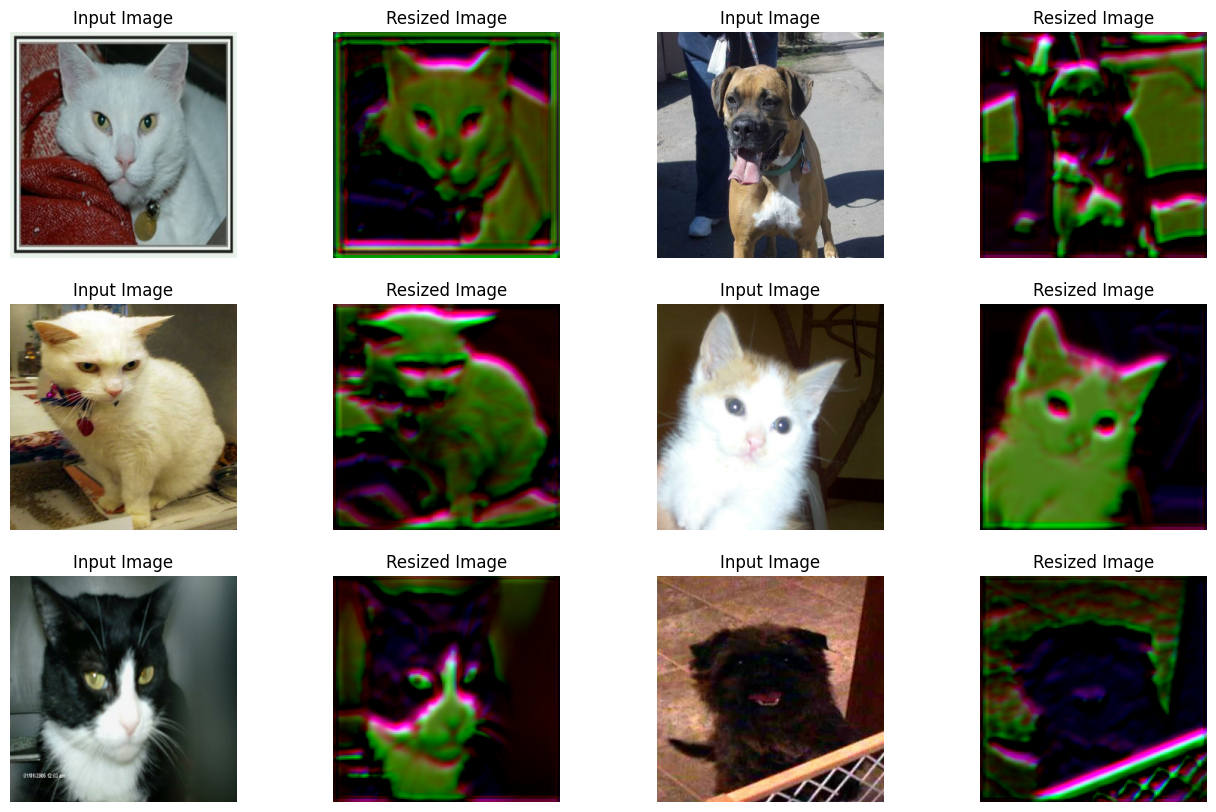
图表显示，经过训练后，图像的视觉效果得到了改善。下表展示了使用缩放模块与使用双线性插值相比的优势：

模型	参数数量（百万）	Top-1 准确率
使用可学习缩放器	7.051717	67.67%
不使用可学习缩放器	7.039554	60.19%

更多详细信息，请查看此仓库。请注意，与本示例不同的是，上面报告的模型在 Cats and Dogs 数据集 90% 的训练集上训练了 10 个 epoch。此外，请注意，由于缩放模块导致的参数数量增加非常微小。为了确保性能提升不是由于随机性造成的，模型是使用相同的初始随机权重进行训练的。

现在，一个值得问的问题是——与基线相比，准确率的提高难道不是仅仅因为给模型添加了更多层（毕竟缩放器是一个迷你网络）的结果吗？

为了表明事实并非如此，作者们进行了以下实验：

取一个在特定尺寸（例如 (224 x 224)）下训练的预训练模型。

现在，首先使用它对缩放到较低分辨率的图像进行推理预测。记录性能。

在第二个实验中，将缩放模块插入预训练模型的顶部，并进行热启动训练。记录性能。

作者们认为，使用第二种选择更好，因为它有助于模型学习如何针对给定分辨率更好地调整表示。由于结果纯粹是经验性的，进行更多实验，例如分析跨通道交互，会更好。值得注意的是，Squeeze and Excitation (SE) 块、Global Context (GC) 块等元素也会为现有网络增加少量参数，但已知它们有助于网络以系统化的方式处理信息，从而提高整体性能。

注释

为了在视觉模型内部引入形状偏见，Geirhos 等人使用自然图像和风格化图像的组合对其进行了训练。由于输出似乎会丢弃纹理信息，研究这个可学习缩放模块是否能实现类似的效果可能会很有趣。

缩放器模块可以处理任意分辨率和纵横比，这对于目标检测和分割等任务非常重要。

另一个密切相关的课题是自适应图像缩放，它试图在训练期间自适应地调整图像/特征图的大小。EfficientV2 就使用了这个想法。