一致性训练(带监督)
作者:Sayak Paul
创建日期 2021/04/13
最后修改日期 2021/04/19
描述: 使用一致性正则化进行训练,以提高模型对数据分布变化的鲁棒性。

当数据独立同分布(i.i.d.)时,深度学习模型在许多图像识别任务中表现出色。然而,当输入数据出现细微的分布变化(如随机噪声、对比度变化和模糊)时,它们的性能可能会下降。因此,自然会产生一个问题:为什么会这样?正如在 A Fourier Perspective on Model Robustness in Computer Vision中所讨论的,深度学习模型没有理由能够抵抗这种变化。标准的模型训练过程(如标准的图像分类训练流程)不会让模型学习超出其在训练数据中看到的知识。
在此示例中,我们将通过以下方式训练一个图像分类模型,并强制其内部产生一种“一致性”:
- 训练一个标准的图像分类模型。
- 在数据集的噪声版本上训练一个相同或更大的模型(使用 RandAugment 进行增强)。
- 为此,我们将首先获取先前模型在数据集的干净图像上的预测。
- 然后,我们将使用这些预测,并在同一图像的噪声变体上训练第二个模型,使其匹配这些预测。这与 知识蒸馏的工作流程相同,但由于学生模型的大小相同或更大,因此此过程也称为自训练。
这个整体的训练流程源于 FixMatch、Unsupervised Data Augmentation for Consistency Training 和 Noisy Student Training 等研究。由于此训练过程鼓励模型对干净和噪声图像产生一致的预测,因此它通常被称为一致性训练或带一致性正则化的训练。尽管本示例侧重于使用一致性训练来增强模型对常见损坏的鲁棒性,但它也可以作为执行弱监督学习的模板。
此示例需要 TensorFlow 2.4 或更高版本,以及 TensorFlow Hub 和 TensorFlow Models,可以使用以下命令进行安装
!pip install -q tf-models-official tensorflow-addons
导入和设置
from official.vision.image_classification.augment import RandAugment
from tensorflow.keras import layers

import tensorflow as tf
import tensorflow_addons as tfa
import matplotlib.pyplot as plt

tf.random.set_seed(42)
定义超参数
AUTO = tf.data.AUTOTUNE
BATCH_SIZE = 128
EPOCHS = 5

CROP_TO = 72
RESIZE_TO = 96
加载 CIFAR-10 数据集
(x_train, y_train), (x_test, y_test) = tf.keras.datasets.cifar10.load_data()

val_samples = 49500
new_train_x, new_y_train = x_train[: val_samples + 1], y_train[: val_samples + 1]
val_x, val_y = x_train[val_samples:], y_train[val_samples:]
创建 TensorFlow Dataset 对象
# Initialize `RandAugment` object with 2 layers of
# augmentation transforms and strength of 9.
augmenter = RandAugment(num_layers=2, magnitude=9)
为了训练教师模型,我们将仅使用两种几何增强变换:随机水平翻转和随机裁剪。
def preprocess_train(image, label, noisy=True):
    image = tf.image.random_flip_left_right(image)
    # We first resize the original image to a larger dimension
    # and then we take random crops from it.
    image = tf.image.resize(image, [RESIZE_TO, RESIZE_TO])
    image = tf.image.random_crop(image, [CROP_TO, CROP_TO, 3])
    if noisy:
        image = augmenter.distort(image)
    return image, label


def preprocess_test(image, label):
    image = tf.image.resize(image, [CROP_TO, CROP_TO])
    return image, label


train_ds = tf.data.Dataset.from_tensor_slices((new_train_x, new_y_train))
validation_ds = tf.data.Dataset.from_tensor_slices((val_x, val_y))
test_ds = tf.data.Dataset.from_tensor_slices((x_test, y_test))
我们确保 train_clean_ds 和 train_noisy_ds 使用*相同*的种子进行洗牌,以确保它们的顺序完全相同。这在训练学生模型时会很有帮助。
# This dataset will be used to train the first model.
train_clean_ds = (
    train_ds.shuffle(BATCH_SIZE * 10, seed=42)
    .map(lambda x, y: (preprocess_train(x, y, noisy=False)), num_parallel_calls=AUTO)
    .batch(BATCH_SIZE)
    .prefetch(AUTO)
)

# This prepares the `Dataset` object to use RandAugment.
train_noisy_ds = (
    train_ds.shuffle(BATCH_SIZE * 10, seed=42)
    .map(preprocess_train, num_parallel_calls=AUTO)
    .batch(BATCH_SIZE)
    .prefetch(AUTO)
)

validation_ds = (
    validation_ds.map(preprocess_test, num_parallel_calls=AUTO)
    .batch(BATCH_SIZE)
    .prefetch(AUTO)
)

test_ds = (
    test_ds.map(preprocess_test, num_parallel_calls=AUTO)
    .batch(BATCH_SIZE)
    .prefetch(AUTO)
)

# This dataset will be used to train the second model.
consistency_training_ds = tf.data.Dataset.zip((train_clean_ds, train_noisy_ds))
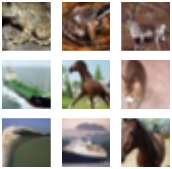
可视化数据集
sample_images, sample_labels = next(iter(train_clean_ds))
plt.figure(figsize=(10, 10))
for i, image in enumerate(sample_images[:9]):
ax = plt.subplot(3, 3, i + 1)
plt.imshow(image.numpy().astype("int"))
plt.axis("off")
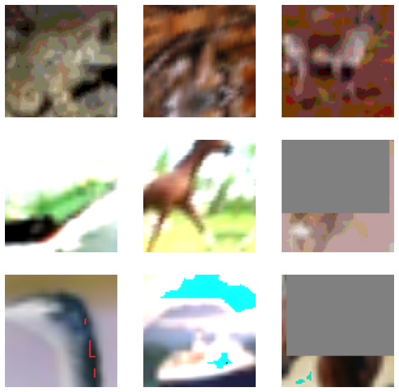
sample_images, sample_labels = next(iter(train_noisy_ds))
plt.figure(figsize=(10, 10))
for i, image in enumerate(sample_images[:9]):
ax = plt.subplot(3, 3, i + 1)
plt.imshow(image.numpy().astype("int"))
plt.axis("off")
定义模型构建实用函数
现在我们定义模型构建实用函数。我们的模型基于 ResNet50V2 架构。
def get_training_model(num_classes=10):
    resnet50_v2 = tf.keras.applications.ResNet50V2(
        weights=None, include_top=False, input_shape=(CROP_TO, CROP_TO, 3),
    )
    model = tf.keras.Sequential(
        [
            layers.Input((CROP_TO, CROP_TO, 3)),
            layers.Rescaling(scale=1.0 / 127.5, offset=-1),
            resnet50_v2,
            layers.GlobalAveragePooling2D(),
            layers.Dense(num_classes),
        ]
    )
    return model
为了可复现性,我们序列化了教师网络的初始随机权重。
initial_teacher_model = get_training_model()
initial_teacher_model.save_weights("initial_teacher_model.h5")
训练教师模型
正如在 Noisy Student Training 中指出的,如果教师模型使用几何集成进行训练,并且学生模型被迫模仿它,这将带来更好的性能。原始论文使用 Stochastic Depth 和 Dropout 来实现集成部分,但在此示例中,我们将使用 Stochastic Weight Averaging (SWA),它也类似于几何集成。
# Define the callbacks.
reduce_lr = tf.keras.callbacks.ReduceLROnPlateau(patience=3)
early_stopping = tf.keras.callbacks.EarlyStopping(
    patience=10, restore_best_weights=True
)

# Initialize SWA from tf-hub.
SWA = tfa.optimizers.SWA

# Compile and train the teacher model.
teacher_model = get_training_model()
teacher_model.load_weights("initial_teacher_model.h5")
teacher_model.compile(
    # Notice that we are wrapping our optimizer within SWA
    optimizer=SWA(tf.keras.optimizers.Adam()),
    loss=tf.keras.losses.SparseCategoricalCrossentropy(from_logits=True),
    metrics=["accuracy"],
)
history = teacher_model.fit(
    train_clean_ds,
    epochs=EPOCHS,
    validation_data=validation_ds,
    callbacks=[reduce_lr, early_stopping],
)

# Evaluate the teacher model on the test set.
_, acc = teacher_model.evaluate(test_ds, verbose=0)
print(f"Test accuracy: {acc*100}%")
Epoch 1/5
387/387 [==============================] - 73s 78ms/step - loss: 1.7785 - accuracy: 0.3582 - val_loss: 2.0589 - val_accuracy: 0.3920
Epoch 2/5
387/387 [==============================] - 28s 71ms/step - loss: 1.2493 - accuracy: 0.5542 - val_loss: 1.4228 - val_accuracy: 0.5380
Epoch 3/5
387/387 [==============================] - 28s 73ms/step - loss: 1.0294 - accuracy: 0.6350 - val_loss: 1.4422 - val_accuracy: 0.5900
Epoch 4/5
387/387 [==============================] - 28s 73ms/step - loss: 0.8954 - accuracy: 0.6864 - val_loss: 1.2189 - val_accuracy: 0.6520
Epoch 5/5
387/387 [==============================] - 28s 73ms/step - loss: 0.7879 - accuracy: 0.7231 - val_loss: 0.9790 - val_accuracy: 0.6500
Test accuracy: 65.83999991416931%
定义自训练实用函数
对于这部分,我们将从 这个 Keras 示例中借用 Distiller 类。
# Majority of the code is taken from:
# https://keras.org.cn/examples/vision/knowledge_distillation/
class SelfTrainer(tf.keras.Model):
    def __init__(self, student, teacher):
        super().__init__()
        self.student = student
        self.teacher = teacher

    def compile(
        self, optimizer, metrics, student_loss_fn, distillation_loss_fn, temperature=3,
    ):
        super().compile(optimizer=optimizer, metrics=metrics)
        self.student_loss_fn = student_loss_fn
        self.distillation_loss_fn = distillation_loss_fn
        self.temperature = temperature

    def train_step(self, data):
        # Since our dataset is a zip of two independent datasets,
        # after initially parsing them, we segregate the
        # respective images and labels next.
        clean_ds, noisy_ds = data
        clean_images, _ = clean_ds
        noisy_images, y = noisy_ds

        # Forward pass of teacher
        teacher_predictions = self.teacher(clean_images, training=False)

        with tf.GradientTape() as tape:
            # Forward pass of student
            student_predictions = self.student(noisy_images, training=True)

            # Compute losses
            student_loss = self.student_loss_fn(y, student_predictions)
            distillation_loss = self.distillation_loss_fn(
                tf.nn.softmax(teacher_predictions / self.temperature, axis=1),
                tf.nn.softmax(student_predictions / self.temperature, axis=1),
            )
            total_loss = (student_loss + distillation_loss) / 2

        # Compute gradients
        trainable_vars = self.student.trainable_variables
        gradients = tape.gradient(total_loss, trainable_vars)

        # Update weights
        self.optimizer.apply_gradients(zip(gradients, trainable_vars))

        # Update the metrics configured in `compile()`
        self.compiled_metrics.update_state(
            y, tf.nn.softmax(student_predictions, axis=1)
        )

        # Return a dict of performance
        results = {m.name: m.result() for m in self.metrics}
        results.update({"total_loss": total_loss})
        return results

    def test_step(self, data):
        # During inference, we only pass a dataset consisting images and labels.
        x, y = data

        # Compute predictions
        y_prediction = self.student(x, training=False)

        # Update the metrics
        self.compiled_metrics.update_state(y, tf.nn.softmax(y_prediction, axis=1))

        # Return a dict of performance
        results = {m.name: m.result() for m in self.metrics}
        return results
此实现中唯一的区别在于损失的计算方式。而不是对蒸馏损失和学生损失进行不同的加权,我们遵循 Noisy Student Training 的方法,取它们的平均值。
训练学生模型
# Define the callbacks.
# We are using a larger decay factor to stabilize the training.
reduce_lr = tf.keras.callbacks.ReduceLROnPlateau(
    patience=3, factor=0.5, monitor="val_accuracy"
)
early_stopping = tf.keras.callbacks.EarlyStopping(
    patience=10, restore_best_weights=True, monitor="val_accuracy"
)

# Compile and train the student model.
self_trainer = SelfTrainer(student=get_training_model(), teacher=teacher_model)
self_trainer.compile(
    # Notice we are *not* using SWA here.
    optimizer="adam",
    metrics=["accuracy"],
    student_loss_fn=tf.keras.losses.SparseCategoricalCrossentropy(from_logits=True),
    distillation_loss_fn=tf.keras.losses.KLDivergence(),
    temperature=10,
)
history = self_trainer.fit(
    consistency_training_ds,
    epochs=EPOCHS,
    validation_data=validation_ds,
    callbacks=[reduce_lr, early_stopping],
)

# Evaluate the student model.
acc = self_trainer.evaluate(test_ds, verbose=0)
print(f"Test accuracy from student model: {acc*100}%")
Epoch 1/5
387/387 [==============================] - 39s 84ms/step - accuracy: 0.2112 - total_loss: 1.0629 - val_accuracy: 0.4180
Epoch 2/5
387/387 [==============================] - 32s 82ms/step - accuracy: 0.3341 - total_loss: 0.9554 - val_accuracy: 0.3900
Epoch 3/5
387/387 [==============================] - 31s 81ms/step - accuracy: 0.3873 - total_loss: 0.8852 - val_accuracy: 0.4580
Epoch 4/5
387/387 [==============================] - 31s 81ms/step - accuracy: 0.4294 - total_loss: 0.8423 - val_accuracy: 0.5660
Epoch 5/5
387/387 [==============================] - 31s 81ms/step - accuracy: 0.4547 - total_loss: 0.8093 - val_accuracy: 0.5880
Test accuracy from student model: 58.490002155303955%
评估模型的鲁棒性
评估视觉模型鲁棒性的标准基准是在 ImageNet-C 和 CIFAR-10-C 等损坏的数据集上记录其性能,这两个数据集均在 Benchmarking Neural Network Robustness to Common Corruptions and Perturbations 中提出。在此示例中,我们将使用 CIFAR-10-C 数据集,该数据集包含 5 个不同严重性级别的 19 种不同损坏。为了评估模型在该数据集上的鲁棒性,我们将执行以下操作:
- 在最高严重性级别运行预训练模型,并获取 Top-1 准确率。
- 计算平均 Top-1 准确率。
出于本示例的目的,我们将不进行这些步骤。这就是为什么我们将模型仅训练了 5 个 epoch。您可以查看 此存储库,其中演示了完整的训练实验以及上述评估。下图展示了该评估的执行摘要。

平均 Top-1 结果代表 CIFAR-10-C 数据集,测试 Top-1 结果代表 CIFAR-10 测试集。很明显,一致性训练不仅在提高模型鲁棒性方面具有优势,而且在提高标准测试性能方面也具有优势。