TPU 上的肺炎分类
作者: Amy MiHyun Jang
创建日期 2020/07/28
最后修改日期 2024/02/12
描述: TPU 上的医学图像分类。

简介 + 设置
本教程将解释如何构建一个 X 射线图像分类模型,以预测 X 射线扫描是否显示肺炎。
import re
import os
import random
import numpy as np
import pandas as pd
import tensorflow as tf
import matplotlib.pyplot as plt

try:
    tpu = tf.distribute.cluster_resolver.TPUClusterResolver.connect()
    print("Device:", tpu.master())
    strategy = tf.distribute.TPUStrategy(tpu)
except:
    strategy = tf.distribute.get_strategy()
print("Number of replicas:", strategy.num_replicas_in_sync)
Device: grpc://10.0.27.122:8470
INFO:tensorflow:Initializing the TPU system: grpc://10.0.27.122:8470

INFO:tensorflow:Initializing the TPU system: grpc://10.0.27.122:8470

INFO:tensorflow:Clearing out eager caches

INFO:tensorflow:Clearing out eager caches

INFO:tensorflow:Finished initializing TPU system.

INFO:tensorflow:Finished initializing TPU system.
WARNING:absl:[`tf.distribute.TPUStrategy`](https://tensorflowcn.cn/api_docs/python/tf/distribute/TPUStrategy) is deprecated, please use  the non experimental symbol [`tf.distribute.TPUStrategy`](https://tensorflowcn.cn/api_docs/python/tf/distribute/TPUStrategy) instead.

INFO:tensorflow:Found TPU system:

INFO:tensorflow:Found TPU system:

INFO:tensorflow:*** Num TPU Cores: 8

INFO:tensorflow:*** Num TPU Cores: 8

INFO:tensorflow:*** Num TPU Workers: 1

INFO:tensorflow:*** Num TPU Workers: 1

INFO:tensorflow:*** Num TPU Cores Per Worker: 8

INFO:tensorflow:*** Num TPU Cores Per Worker: 8

INFO:tensorflow:*** Available Device: _DeviceAttributes(/job:localhost/replica:0/task:0/device:CPU:0, CPU, 0, 0)

INFO:tensorflow:*** Available Device: _DeviceAttributes(/job:localhost/replica:0/task:0/device:CPU:0, CPU, 0, 0)

INFO:tensorflow:*** Available Device: _DeviceAttributes(/job:localhost/replica:0/task:0/device:XLA_CPU:0, XLA_CPU, 0, 0)

INFO:tensorflow:*** Available Device: _DeviceAttributes(/job:localhost/replica:0/task:0/device:XLA_CPU:0, XLA_CPU, 0, 0)

INFO:tensorflow:*** Available Device: _DeviceAttributes(/job:worker/replica:0/task:0/device:CPU:0, CPU, 0, 0)

INFO:tensorflow:*** Available Device: _DeviceAttributes(/job:worker/replica:0/task:0/device:CPU:0, CPU, 0, 0)

INFO:tensorflow:*** Available Device: _DeviceAttributes(/job:worker/replica:0/task:0/device:TPU:0, TPU, 0, 0)

INFO:tensorflow:*** Available Device: _DeviceAttributes(/job:worker/replica:0/task:0/device:TPU:0, TPU, 0, 0)

INFO:tensorflow:*** Available Device: _DeviceAttributes(/job:worker/replica:0/task:0/device:TPU:1, TPU, 0, 0)

INFO:tensorflow:*** Available Device: _DeviceAttributes(/job:worker/replica:0/task:0/device:TPU:1, TPU, 0, 0)

INFO:tensorflow:*** Available Device: _DeviceAttributes(/job:worker/replica:0/task:0/device:TPU:2, TPU, 0, 0)

INFO:tensorflow:*** Available Device: _DeviceAttributes(/job:worker/replica:0/task:0/device:TPU:2, TPU, 0, 0)

INFO:tensorflow:*** Available Device: _DeviceAttributes(/job:worker/replica:0/task:0/device:TPU:3, TPU, 0, 0)

INFO:tensorflow:*** Available Device: _DeviceAttributes(/job:worker/replica:0/task:0/device:TPU:3, TPU, 0, 0)

INFO:tensorflow:*** Available Device: _DeviceAttributes(/job:worker/replica:0/task:0/device:TPU:4, TPU, 0, 0)

INFO:tensorflow:*** Available Device: _DeviceAttributes(/job:worker/replica:0/task:0/device:TPU:4, TPU, 0, 0)

INFO:tensorflow:*** Available Device: _DeviceAttributes(/job:worker/replica:0/task:0/device:TPU:5, TPU, 0, 0)

INFO:tensorflow:*** Available Device: _DeviceAttributes(/job:worker/replica:0/task:0/device:TPU:5, TPU, 0, 0)

INFO:tensorflow:*** Available Device: _DeviceAttributes(/job:worker/replica:0/task:0/device:TPU:6, TPU, 0, 0)

INFO:tensorflow:*** Available Device: _DeviceAttributes(/job:worker/replica:0/task:0/device:TPU:6, TPU, 0, 0)

INFO:tensorflow:*** Available Device: _DeviceAttributes(/job:worker/replica:0/task:0/device:TPU:7, TPU, 0, 0)

INFO:tensorflow:*** Available Device: _DeviceAttributes(/job:worker/replica:0/task:0/device:TPU:7, TPU, 0, 0)

INFO:tensorflow:*** Available Device: _DeviceAttributes(/job:worker/replica:0/task:0/device:TPU_SYSTEM:0, TPU_SYSTEM, 0, 0)

INFO:tensorflow:*** Available Device: _DeviceAttributes(/job:worker/replica:0/task:0/device:TPU_SYSTEM:0, TPU_SYSTEM, 0, 0)

INFO:tensorflow:*** Available Device: _DeviceAttributes(/job:worker/replica:0/task:0/device:XLA_CPU:0, XLA_CPU, 0, 0)

INFO:tensorflow:*** Available Device: _DeviceAttributes(/job:worker/replica:0/task:0/device:XLA_CPU:0, XLA_CPU, 0, 0)

Number of replicas: 8
我们需要一个指向我们数据的 Google Cloud 链接,以便使用 TPU 加载数据。下面,我们定义了将在本示例中使用的关键配置参数。要在 TPU 上运行,此示例必须位于 Colab 中并选择 TPU 运行时。
AUTOTUNE = tf.data.AUTOTUNE
BATCH_SIZE = 25 * strategy.num_replicas_in_sync
IMAGE_SIZE = [180, 180]
CLASS_NAMES = ["NORMAL", "PNEUMONIA"]
加载数据
我们正在使用的来自 Cell 的胸部 X 射线数据将数据分为训练集和测试集。让我们首先加载训练 TFRecords。
train_images = tf.data.TFRecordDataset(
    "gs://download.tensorflow.org/data/ChestXRay2017/train/images.tfrec"
)
train_paths = tf.data.TFRecordDataset(
    "gs://download.tensorflow.org/data/ChestXRay2017/train/paths.tfrec"
)

ds = tf.data.Dataset.zip((train_images, train_paths))
让我们计算一下我们有多少健康/正常的胸部 X 射线以及多少肺炎胸部 X 射线。
COUNT_NORMAL = len(
    [
        filename
        for filename in train_paths
        if "NORMAL" in filename.numpy().decode("utf-8")
    ]
)
print("Normal images count in training set: " + str(COUNT_NORMAL))

COUNT_PNEUMONIA = len(
    [
        filename
        for filename in train_paths
        if "PNEUMONIA" in filename.numpy().decode("utf-8")
    ]
)
print("Pneumonia images count in training set: " + str(COUNT_PNEUMONIA))
Normal images count in training set: 1349
Pneumonia images count in training set: 3883
请注意,分类为肺炎的图像比正常的要多得多。这表明我们的数据不平衡。我们将在笔记本的后续部分解决这种不平衡问题。
我们希望将每个文件名映射到相应的 (图像, 标签) 对。以下方法将帮助我们做到这一点。
由于我们只有两个标签,我们将对标签进行编码,其中 1 或 True 表示肺炎,0 或 False 表示正常。
def get_label(file_path):
    # convert the path to a list of path components
    parts = tf.strings.split(file_path, "/")
    # The second to last is the class-directory
    if parts[-2] == "PNEUMONIA":
        return 1
    else:
        return 0


def decode_img(img):
    # convert the compressed string to a 3D uint8 tensor
    img = tf.image.decode_jpeg(img, channels=3)
    # resize the image to the desired size.
    return tf.image.resize(img, IMAGE_SIZE)


def process_path(image, path):
    label = get_label(path)
    # load the raw data from the file as a string
    img = decode_img(image)
    return img, label


ds = ds.map(process_path, num_parallel_calls=AUTOTUNE)
让我们将数据分为训练集和验证集。
ds = ds.shuffle(10000)
train_ds = ds.take(4200)
val_ds = ds.skip(4200)
让我们可视化 (图像, 标签) 对的形状。
for image, label in train_ds.take(1):
    print("Image shape: ", image.numpy().shape)
    print("Label: ", label.numpy())
Image shape:  (180, 180, 3)
Label:  False
加载并格式化测试数据。
test_images = tf.data.TFRecordDataset(
    "gs://download.tensorflow.org/data/ChestXRay2017/test/images.tfrec"
)
test_paths = tf.data.TFRecordDataset(
    "gs://download.tensorflow.org/data/ChestXRay2017/test/paths.tfrec"
)
test_ds = tf.data.Dataset.zip((test_images, test_paths))

test_ds = test_ds.map(process_path, num_parallel_calls=AUTOTUNE)
test_ds = test_ds.batch(BATCH_SIZE)
可视化数据集
首先,让我们使用缓冲预取,这样我们就可以从磁盘生成数据,而不会出现 I/O 阻塞。
请注意,大型图像数据集不应缓存在内存中。我们在这里这样做是因为数据集不是很大,并且我们想在 TPU 上进行训练。
def prepare_for_training(ds, cache=True):
    # This is a small dataset, only load it once, and keep it in memory.
    # use `.cache(filename)` to cache preprocessing work for datasets that don't
    # fit in memory.
    if cache:
        if isinstance(cache, str):
            ds = ds.cache(cache)
        else:
            ds = ds.cache()

    ds = ds.batch(BATCH_SIZE)

    # `prefetch` lets the dataset fetch batches in the background while the model
    # is training.
    ds = ds.prefetch(buffer_size=AUTOTUNE)

    return ds
调用训练数据的下一个批次迭代。
train_ds = prepare_for_training(train_ds)
val_ds = prepare_for_training(val_ds)

image_batch, label_batch = next(iter(train_ds))
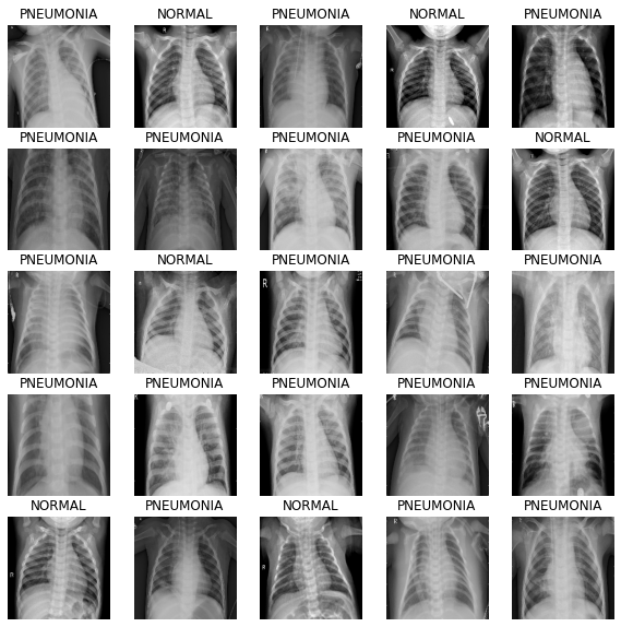
定义显示批次中图像的方法。
def show_batch(image_batch, label_batch):
    plt.figure(figsize=(10, 10))
    for n in range(25):
        ax = plt.subplot(5, 5, n + 1)
        plt.imshow(image_batch[n] / 255)
        if label_batch[n]:
            plt.title("PNEUMONIA")
        else:
            plt.title("NORMAL")
        plt.axis("off")
由于该方法将其参数作为 NumPy 数组,因此在批次上调用 numpy 函数以 NumPy 数组形式返回张量。
show_batch(image_batch.numpy(), label_batch.numpy())
构建 CNN
为了使我们的模型更具模块化和易于理解,让我们定义一些块。由于我们正在构建卷积神经网络,因此我们将创建一个卷积块和一个密集层块。
此 CNN 的架构受到这篇 文章 的启发。
import os
os.environ['KERAS_BACKEND'] = 'tensorflow'

import keras
from keras import layers

def conv_block(filters, inputs):
    x = layers.SeparableConv2D(filters, 3, activation="relu", padding="same")(inputs)
    x = layers.SeparableConv2D(filters, 3, activation="relu", padding="same")(x)
    x = layers.BatchNormalization()(x)
    outputs = layers.MaxPool2D()(x)

    return outputs


def dense_block(units, dropout_rate, inputs):
    x = layers.Dense(units, activation="relu")(inputs)
    x = layers.BatchNormalization()(x)
    outputs = layers.Dropout(dropout_rate)(x)

    return outputs
以下方法将定义一个函数来为我们构建模型。
图像的原始值范围是 [0, 255]。CNN 在处理较小的数字时效果更好,因此我们将输入值缩减。
Dropout 层很重要,因为它们降低了模型过拟合的可能性。我们希望在模型的末尾设置一个具有一个节点的 Dense 层,因为这将是确定 X 射线是否显示肺炎的二元输出。
def build_model():
    inputs = keras.Input(shape=(IMAGE_SIZE[0], IMAGE_SIZE[1], 3))
    x = layers.Rescaling(1.0 / 255)(inputs)
    x = layers.Conv2D(16, 3, activation="relu", padding="same")(x)
    x = layers.Conv2D(16, 3, activation="relu", padding="same")(x)
    x = layers.MaxPool2D()(x)

    x = conv_block(32, x)
    x = conv_block(64, x)

    x = conv_block(128, x)
    x = layers.Dropout(0.2)(x)

    x = conv_block(256, x)
    x = layers.Dropout(0.2)(x)

    x = layers.Flatten()(x)
    x = dense_block(512, 0.7, x)
    x = dense_block(128, 0.5, x)
    x = dense_block(64, 0.3, x)

    outputs = layers.Dense(1, activation="sigmoid")(x)

    model = keras.Model(inputs=inputs, outputs=outputs)
    return model
纠正数据不平衡
我们在本示例前面已经看到数据不平衡,肺炎图像多于正常图像。我们将通过使用类权重来纠正这一点。
initial_bias = np.log([COUNT_PNEUMONIA / COUNT_NORMAL])
print("Initial bias: {:.5f}".format(initial_bias[0]))

TRAIN_IMG_COUNT = COUNT_NORMAL + COUNT_PNEUMONIA
weight_for_0 = (1 / COUNT_NORMAL) * (TRAIN_IMG_COUNT) / 2.0
weight_for_1 = (1 / COUNT_PNEUMONIA) * (TRAIN_IMG_COUNT) / 2.0

class_weight = {0: weight_for_0, 1: weight_for_1}

print("Weight for class 0: {:.2f}".format(weight_for_0))
print("Weight for class 1: {:.2f}".format(weight_for_1))
Initial bias: 1.05724
Weight for class 0: 1.94
Weight for class 1: 0.67
类别 0 (正常) 的权重远高于类别 1 (肺炎) 的权重。由于正常的图像较少,每个正常图像的权重会更大,以平衡数据,因为 CNN 在训练数据平衡时效果最好。
训练模型
定义回调
检查点回调会保存模型的最佳权重,因此下次我们想使用模型时,无需花费时间进行训练。当模型开始停滞,甚至更糟,当模型开始过拟合时,提前停止回调会停止训练过程。
checkpoint_cb = keras.callbacks.ModelCheckpoint("xray_model.keras", save_best_only=True)

early_stopping_cb = keras.callbacks.EarlyStopping(
    patience=10, restore_best_weights=True
)
我们还想调整学习率。过高的学习率会导致模型发散。过小的学习率会导致模型过慢。我们在下面实现了指数学习率调度方法。
initial_learning_rate = 0.015
lr_schedule = keras.optimizers.schedules.ExponentialDecay(
    initial_learning_rate, decay_steps=100000, decay_rate=0.96, staircase=True
)
拟合模型
对于我们的指标,我们希望包含精确率和召回率,因为它们将为我们提供有关模型有多好的更具信息量的图景。准确率告诉我们正确标签的比例。由于我们的数据不平衡,准确率可能会给人一种好模型的错觉(例如,一个总是预测“肺炎”的模型将具有 74% 的准确率,但它不是一个好模型)。
精确率是真正例 (TP) 除以 TP 和假正例 (FP) 之和。它显示了标记为正例的样本中有多少是实际正确的。
召回率是 TP 除以 TP 和假负例 (FN) 之和。它显示了实际正例中有多少是正确的。
由于图像只有两个可能的标签,我们将使用二元交叉熵损失。在拟合模型时,请记住指定我们之前定义的类权重。由于我们正在使用 TPU,训练将很快完成 - 少于 2 分钟。
with strategy.scope():
    model = build_model()

    METRICS = [
        keras.metrics.BinaryAccuracy(),
        keras.metrics.Precision(name="precision"),
        keras.metrics.Recall(name="recall"),
    ]
    model.compile(
        optimizer=keras.optimizers.Adam(learning_rate=lr_schedule),
        loss="binary_crossentropy",
        metrics=METRICS,
    )

history = model.fit(
    train_ds,
    epochs=100,
    validation_data=val_ds,
    class_weight=class_weight,
    callbacks=[checkpoint_cb, early_stopping_cb],
)
Epoch 1/100
WARNING:tensorflow:From /usr/local/lib/python3.6/dist-packages/tensorflow/python/data/ops/multi_device_iterator_ops.py:601: get_next_as_optional (from tensorflow.python.data.ops.iterator_ops) is deprecated and will be removed in a future version.
Instructions for updating:
Use `tf.data.Iterator.get_next_as_optional()` instead.

21/21 [==============================] - 12s 568ms/step - loss: 0.5857 - binary_accuracy: 0.6960 - precision: 0.8887 - recall: 0.6733 - val_loss: 34.0149 - val_binary_accuracy: 0.7180 - val_precision: 0.7180 - val_recall: 1.0000
Epoch 2/100
21/21 [==============================] - 3s 128ms/step - loss: 0.2916 - binary_accuracy: 0.8755 - precision: 0.9540 - recall: 0.8738 - val_loss: 97.5194 - val_binary_accuracy: 0.7180 - val_precision: 0.7180 - val_recall: 1.0000
Epoch 3/100
21/21 [==============================] - 4s 167ms/step - loss: 0.2384 - binary_accuracy: 0.9002 - precision: 0.9663 - recall: 0.8964 - val_loss: 27.7902 - val_binary_accuracy: 0.7180 - val_precision: 0.7180 - val_recall: 1.0000
Epoch 4/100
21/21 [==============================] - 4s 173ms/step - loss: 0.2046 - binary_accuracy: 0.9145 - precision: 0.9725 - recall: 0.9102 - val_loss: 10.8302 - val_binary_accuracy: 0.7180 - val_precision: 0.7180 - val_recall: 1.0000
Epoch 5/100
21/21 [==============================] - 4s 174ms/step - loss: 0.1841 - binary_accuracy: 0.9279 - precision: 0.9733 - recall: 0.9279 - val_loss: 3.5860 - val_binary_accuracy: 0.7103 - val_precision: 0.7162 - val_recall: 0.9879
Epoch 6/100
21/21 [==============================] - 4s 185ms/step - loss: 0.1600 - binary_accuracy: 0.9362 - precision: 0.9791 - recall: 0.9337 - val_loss: 0.3014 - val_binary_accuracy: 0.8895 - val_precision: 0.8973 - val_recall: 0.9555
Epoch 7/100
21/21 [==============================] - 3s 130ms/step - loss: 0.1567 - binary_accuracy: 0.9393 - precision: 0.9798 - recall: 0.9372 - val_loss: 0.6763 - val_binary_accuracy: 0.7810 - val_precision: 0.7760 - val_recall: 0.9771
Epoch 8/100
21/21 [==============================] - 3s 131ms/step - loss: 0.1532 - binary_accuracy: 0.9421 - precision: 0.9825 - recall: 0.9385 - val_loss: 0.3169 - val_binary_accuracy: 0.8895 - val_precision: 0.8684 - val_recall: 0.9973
Epoch 9/100
21/21 [==============================] - 4s 184ms/step - loss: 0.1457 - binary_accuracy: 0.9431 - precision: 0.9822 - recall: 0.9401 - val_loss: 0.2064 - val_binary_accuracy: 0.9273 - val_precision: 0.9840 - val_recall: 0.9136
Epoch 10/100
21/21 [==============================] - 3s 132ms/step - loss: 0.1201 - binary_accuracy: 0.9521 - precision: 0.9869 - recall: 0.9479 - val_loss: 0.4364 - val_binary_accuracy: 0.8605 - val_precision: 0.8443 - val_recall: 0.9879
Epoch 11/100
21/21 [==============================] - 3s 127ms/step - loss: 0.1200 - binary_accuracy: 0.9510 - precision: 0.9863 - recall: 0.9469 - val_loss: 0.5197 - val_binary_accuracy: 0.8508 - val_precision: 1.0000 - val_recall: 0.7922
Epoch 12/100
21/21 [==============================] - 4s 186ms/step - loss: 0.1077 - binary_accuracy: 0.9581 - precision: 0.9870 - recall: 0.9559 - val_loss: 0.1349 - val_binary_accuracy: 0.9486 - val_precision: 0.9587 - val_recall: 0.9703
Epoch 13/100
21/21 [==============================] - 4s 173ms/step - loss: 0.0918 - binary_accuracy: 0.9650 - precision: 0.9914 - recall: 0.9611 - val_loss: 0.0926 - val_binary_accuracy: 0.9700 - val_precision: 0.9837 - val_recall: 0.9744
Epoch 14/100
21/21 [==============================] - 3s 130ms/step - loss: 0.0996 - binary_accuracy: 0.9612 - precision: 0.9913 - recall: 0.9559 - val_loss: 0.1811 - val_binary_accuracy: 0.9419 - val_precision: 0.9956 - val_recall: 0.9231
Epoch 15/100
21/21 [==============================] - 3s 129ms/step - loss: 0.0898 - binary_accuracy: 0.9643 - precision: 0.9901 - recall: 0.9614 - val_loss: 0.1525 - val_binary_accuracy: 0.9486 - val_precision: 0.9986 - val_recall: 0.9298
Epoch 16/100
21/21 [==============================] - 3s 128ms/step - loss: 0.0941 - binary_accuracy: 0.9621 - precision: 0.9904 - recall: 0.9582 - val_loss: 0.5101 - val_binary_accuracy: 0.8527 - val_precision: 1.0000 - val_recall: 0.7949
Epoch 17/100
21/21 [==============================] - 3s 125ms/step - loss: 0.0798 - binary_accuracy: 0.9636 - precision: 0.9897 - recall: 0.9607 - val_loss: 0.1239 - val_binary_accuracy: 0.9622 - val_precision: 0.9875 - val_recall: 0.9595
Epoch 18/100
21/21 [==============================] - 3s 126ms/step - loss: 0.0821 - binary_accuracy: 0.9657 - precision: 0.9911 - recall: 0.9623 - val_loss: 0.1597 - val_binary_accuracy: 0.9322 - val_precision: 0.9956 - val_recall: 0.9096
Epoch 19/100
21/21 [==============================] - 3s 143ms/step - loss: 0.0800 - binary_accuracy: 0.9657 - precision: 0.9917 - recall: 0.9617 - val_loss: 0.2538 - val_binary_accuracy: 0.9109 - val_precision: 1.0000 - val_recall: 0.8758
Epoch 20/100
21/21 [==============================] - 3s 127ms/step - loss: 0.0605 - binary_accuracy: 0.9738 - precision: 0.9950 - recall: 0.9694 - val_loss: 0.6594 - val_binary_accuracy: 0.8566 - val_precision: 1.0000 - val_recall: 0.8003
Epoch 21/100
21/21 [==============================] - 4s 167ms/step - loss: 0.0726 - binary_accuracy: 0.9733 - precision: 0.9937 - recall: 0.9701 - val_loss: 0.0593 - val_binary_accuracy: 0.9816 - val_precision: 0.9945 - val_recall: 0.9798
Epoch 22/100
21/21 [==============================] - 3s 126ms/step - loss: 0.0577 - binary_accuracy: 0.9783 - precision: 0.9951 - recall: 0.9755 - val_loss: 0.1087 - val_binary_accuracy: 0.9729 - val_precision: 0.9931 - val_recall: 0.9690
Epoch 23/100
21/21 [==============================] - 3s 125ms/step - loss: 0.0652 - binary_accuracy: 0.9729 - precision: 0.9924 - recall: 0.9707 - val_loss: 1.8465 - val_binary_accuracy: 0.7180 - val_precision: 0.7180 - val_recall: 1.0000
Epoch 24/100
21/21 [==============================] - 3s 124ms/step - loss: 0.0538 - binary_accuracy: 0.9783 - precision: 0.9951 - recall: 0.9755 - val_loss: 1.5769 - val_binary_accuracy: 0.7180 - val_precision: 0.7180 - val_recall: 1.0000
Epoch 25/100
21/21 [==============================] - 4s 167ms/step - loss: 0.0549 - binary_accuracy: 0.9776 - precision: 0.9954 - recall: 0.9743 - val_loss: 0.0590 - val_binary_accuracy: 0.9777 - val_precision: 0.9904 - val_recall: 0.9784
Epoch 26/100
21/21 [==============================] - 3s 131ms/step - loss: 0.0677 - binary_accuracy: 0.9719 - precision: 0.9924 - recall: 0.9694 - val_loss: 2.6008 - val_binary_accuracy: 0.6928 - val_precision: 0.9977 - val_recall: 0.5735
Epoch 27/100
21/21 [==============================] - 3s 127ms/step - loss: 0.0469 - binary_accuracy: 0.9833 - precision: 0.9971 - recall: 0.9804 - val_loss: 1.0184 - val_binary_accuracy: 0.8605 - val_precision: 0.9983 - val_recall: 0.8070
Epoch 28/100
21/21 [==============================] - 3s 126ms/step - loss: 0.0501 - binary_accuracy: 0.9790 - precision: 0.9961 - recall: 0.9755 - val_loss: 0.3737 - val_binary_accuracy: 0.9089 - val_precision: 0.9954 - val_recall: 0.8772
Epoch 29/100
21/21 [==============================] - 3s 128ms/step - loss: 0.0548 - binary_accuracy: 0.9798 - precision: 0.9941 - recall: 0.9784 - val_loss: 1.2928 - val_binary_accuracy: 0.7907 - val_precision: 1.0000 - val_recall: 0.7085
Epoch 30/100
21/21 [==============================] - 3s 129ms/step - loss: 0.0370 - binary_accuracy: 0.9860 - precision: 0.9980 - recall: 0.9829 - val_loss: 0.1370 - val_binary_accuracy: 0.9612 - val_precision: 0.9972 - val_recall: 0.9487
Epoch 31/100
21/21 [==============================] - 3s 125ms/step - loss: 0.0585 - binary_accuracy: 0.9819 - precision: 0.9951 - recall: 0.9804 - val_loss: 1.1955 - val_binary_accuracy: 0.6870 - val_precision: 0.9976 - val_recall: 0.5655
Epoch 32/100
21/21 [==============================] - 3s 140ms/step - loss: 0.0813 - binary_accuracy: 0.9695 - precision: 0.9934 - recall: 0.9652 - val_loss: 1.0394 - val_binary_accuracy: 0.8576 - val_precision: 0.9853 - val_recall: 0.8138
Epoch 33/100
21/21 [==============================] - 3s 128ms/step - loss: 0.1111 - binary_accuracy: 0.9555 - precision: 0.9870 - recall: 0.9524 - val_loss: 4.9438 - val_binary_accuracy: 0.5911 - val_precision: 1.0000 - val_recall: 0.4305
Epoch 34/100
21/21 [==============================] - 3s 130ms/step - loss: 0.0680 - binary_accuracy: 0.9726 - precision: 0.9921 - recall: 0.9707 - val_loss: 2.8822 - val_binary_accuracy: 0.7267 - val_precision: 0.9978 - val_recall: 0.6208
Epoch 35/100
21/21 [==============================] - 4s 187ms/step - loss: 0.0784 - binary_accuracy: 0.9712 - precision: 0.9892 - recall: 0.9717 - val_loss: 0.3940 - val_binary_accuracy: 0.9390 - val_precision: 0.9942 - val_recall: 0.9204
可视化模型性能
让我们绘制训练集和验证集的模型准确率和损失。请注意,此笔记本未指定随机种子。对于您的笔记本,可能会有轻微的差异。
fig, ax = plt.subplots(1, 4, figsize=(20, 3))
ax = ax.ravel()

for i, met in enumerate(["precision", "recall", "binary_accuracy", "loss"]):
    ax[i].plot(history.history[met])
    ax[i].plot(history.history["val_" + met])
    ax[i].set_title("Model {}".format(met))
    ax[i].set_xlabel("epochs")
    ax[i].set_ylabel(met)
    ax[i].legend(["train", "val"])
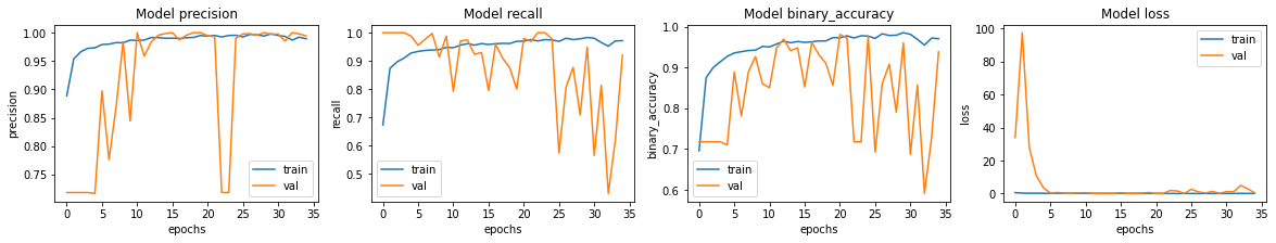
我们看到我们模型的准确率约为 95%。
预测和评估结果
让我们在我们的测试数据上评估模型!
model.evaluate(test_ds, return_dict=True)
4/4 [==============================] - 3s 708ms/step - loss: 0.9718 - binary_accuracy: 0.7901 - precision: 0.7524 - recall: 0.9897

{'binary_accuracy': 0.7900640964508057,
 'loss': 0.9717951416969299,
 'precision': 0.752436637878418,
 'recall': 0.9897436499595642}
我们看到我们在测试数据上的准确率低于我们在验证集上的准确率。这可能表明过拟合。
我们的召回率高于我们的精确率,这表明几乎所有肺炎图像都能被正确识别,但一些正常图像被错误地识别。我们应该努力提高我们的精确率。
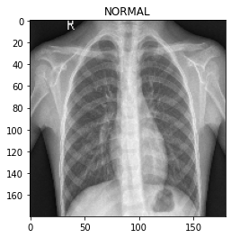
for image, label in test_ds.take(1):
    plt.imshow(image[0] / 255.0)
    plt.title(CLASS_NAMES[label[0].numpy()])

prediction = model.predict(test_ds.take(1))[0]
scores = [1 - prediction, prediction]

for score, name in zip(scores, CLASS_NAMES):
    print("This image is %.2f percent %s" % ((100 * score), name))
/usr/local/lib/python3.6/dist-packages/ipykernel_launcher.py:3: DeprecationWarning: In future, it will be an error for 'np.bool_' scalars to be interpreted as an index
  This is separate from the ipykernel package so we can avoid doing imports until

This image is 47.19 percent NORMAL
This image is 52.81 percent PNEUMONIA