无
可视化卷积网络学习的内容
作者: fchollet
创建日期 2020/05/29
最后修改日期 2020/05/29
描述: 显示卷积网络滤波器响应的视觉模式。

简介
在此示例中,我们将深入研究图像分类模型学习到的视觉模式。我们将使用在 ImageNet 数据集上训练的 ResNet50V2 模型。
我们的过程很简单:我们将创建输入图像,以最大化目标层(选择在模型中间位置:层 conv3_block4_out)中特定滤波器的激活。这些图像代表了滤波器响应的模式的可视化。
设置
import os

os.environ["KERAS_BACKEND"] = "tensorflow"

import keras
import numpy as np
import tensorflow as tf

# The dimensions of our input image
img_width = 180
img_height = 180
# Our target layer: we will visualize the filters from this layer.
# See `model.summary()` for list of layer names, if you want to change this.
layer_name = "conv3_block4_out"
构建特征提取模型
# Build a ResNet50V2 model loaded with pre-trained ImageNet weights
model = keras.applications.ResNet50V2(weights="imagenet", include_top=False)

# Set up a model that returns the activation values for our target layer
layer = model.get_layer(name=layer_name)
feature_extractor = keras.Model(inputs=model.inputs, outputs=layer.output)
设置梯度上升过程
我们将最大化的“损失”简单地是目标层中特定滤波器的激活的平均值。为避免边界效应,我们排除了边界像素。
def compute_loss(input_image, filter_index):
    activation = feature_extractor(input_image)
    # We avoid border artifacts by only involving non-border pixels in the loss.
    filter_activation = activation[:, 2:-2, 2:-2, filter_index]
    return tf.reduce_mean(filter_activation)
我们的梯度上升函数简单地计算损失(如上)相对于输入图像的梯度,并更新图像,使其朝着更强地激活目标滤波器的状态移动。
@tf.function
def gradient_ascent_step(img, filter_index, learning_rate):
    with tf.GradientTape() as tape:
        tape.watch(img)
        loss = compute_loss(img, filter_index)
    # Compute gradients.
    grads = tape.gradient(loss, img)
    # Normalize gradients.
    grads = tf.math.l2_normalize(grads)
    img += learning_rate * grads
    return loss, img
设置端到端滤波器可视化循环
我们的过程如下:
- 从一个接近“全灰色”(即视觉上中性)的随机图像开始
- 重复应用上面定义的梯度上升步函数
- 通过标准化、中心裁剪并将结果输入图像限制在 [0, 255] 范围内,将其转换回可显示的形式。
def initialize_image():
    # We start from a gray image with some random noise
    img = tf.random.uniform((1, img_width, img_height, 3))
    # ResNet50V2 expects inputs in the range [-1, +1].
    # Here we scale our random inputs to [-0.125, +0.125]
    return (img - 0.5) * 0.25


def visualize_filter(filter_index):
    # We run gradient ascent for 20 steps
    iterations = 30
    learning_rate = 10.0
    img = initialize_image()
    for iteration in range(iterations):
        loss, img = gradient_ascent_step(img, filter_index, learning_rate)

    # Decode the resulting input image
    img = deprocess_image(img[0].numpy())
    return loss, img


def deprocess_image(img):
    # Normalize array: center on 0., ensure variance is 0.15
    img -= img.mean()
    img /= img.std() + 1e-5
    img *= 0.15

    # Center crop
    img = img[25:-25, 25:-25, :]

    # Clip to [0, 1]
    img += 0.5
    img = np.clip(img, 0, 1)

    # Convert to RGB array
    img *= 255
    img = np.clip(img, 0, 255).astype("uint8")
    return img
让我们尝试使用目标层中的滤波器 0 进行测试
from IPython.display import Image, display

loss, img = visualize_filter(0)
keras.utils.save_img("0.png", img)
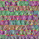
这就是最大化目标层中滤波器 0 响应的输入图像的样子
display(Image("0.png"))
可视化目标层中的前 64 个滤波器
现在,让我们制作目标层中前 64 个滤波器的 8x8 网格,以了解模型学习到的各种视觉模式的范围。
# Compute image inputs that maximize per-filter activations
# for the first 64 filters of our target layer
all_imgs = []
for filter_index in range(64):
    print("Processing filter %d" % (filter_index,))
    loss, img = visualize_filter(filter_index)
    all_imgs.append(img)

# Build a black picture with enough space for
# our 8 x 8 filters of size 128 x 128, with a 5px margin in between
margin = 5
n = 8
cropped_width = img_width - 25 * 2
cropped_height = img_height - 25 * 2
width = n * cropped_width + (n - 1) * margin
height = n * cropped_height + (n - 1) * margin
stitched_filters = np.zeros((width, height, 3))

# Fill the picture with our saved filters
for i in range(n):
    for j in range(n):
        img = all_imgs[i * n + j]
        stitched_filters[
            (cropped_width + margin) * i : (cropped_width + margin) * i + cropped_width,
            (cropped_height + margin) * j : (cropped_height + margin) * j
            + cropped_height,
            :,
        ] = img
keras.utils.save_img("stiched_filters.png", stitched_filters)

from IPython.display import Image, display

display(Image("stiched_filters.png"))
Processing filter 0
Processing filter 1
Processing filter 2
Processing filter 3
Processing filter 4
Processing filter 5
Processing filter 6
Processing filter 7
Processing filter 8
Processing filter 9
Processing filter 10
Processing filter 11
Processing filter 12
Processing filter 13
Processing filter 14
Processing filter 15
Processing filter 16
Processing filter 17
Processing filter 18
Processing filter 19
Processing filter 20
Processing filter 21
Processing filter 22
Processing filter 23
Processing filter 24
Processing filter 25
Processing filter 26
Processing filter 27
Processing filter 28
Processing filter 29
Processing filter 30
Processing filter 31
Processing filter 32
Processing filter 33
Processing filter 34
Processing filter 35
Processing filter 36
Processing filter 37
Processing filter 38
Processing filter 39
Processing filter 40
Processing filter 41
Processing filter 42
Processing filter 43
Processing filter 44
Processing filter 45
Processing filter 46
Processing filter 47
Processing filter 48
Processing filter 49
Processing filter 50
Processing filter 51
Processing filter 52
Processing filter 53
Processing filter 54
Processing filter 55
Processing filter 56
Processing filter 57
Processing filter 58
Processing filter 59
Processing filter 60
Processing filter 61
Processing filter 62
Processing filter 63
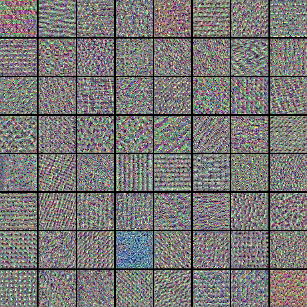
图像分类模型通过分解输入到诸如这些之类的纹理滤波器的“向量基”来观察世界。
有关分析和解释,请参阅 这篇旧博客文章。