使用 SimSiam 进行自监督对比学习
作者:Sayak Paul
创建日期 2021/03/19
最后修改日期 2023/12/29
描述: 计算机视觉自监督学习方法的实现。

自监督学习(SSL)是表示学习领域一个有趣的研究分支。SSL 系统尝试从无标签数据点语料库中构建监督信号。一个例子是训练一个深度神经网络,使其能够根据给定的词语集合预测下一个词。在文献中,这些任务被称为预置任务或辅助任务。如果我们 在海量数据集(例如 维基百科文本语料库)上训练这样的网络,它就能学到非常有效的表示,这些表示能够很好地迁移到下游任务。像 BERT、GPT-3、ELMo 这样的语言模型都受益于此。
与语言模型非常相似,我们也可以使用类似的方法来训练计算机视觉模型。为了在计算机视觉领域奏效,我们需要构建学习任务,以便底层模型(深度神经网络)能够理解视觉数据中存在的语义信息。其中一项任务是让模型对同一图像的两个不同版本进行对比。希望通过这种方式,模型能够学习到将相似图像尽可能地聚集在一起,同时将不相似图像分开的表示。
在本例中,我们将实现一个名为 **SimSiam** 的系统,该系统在 《Exploring Simple Siamese Representation Learning》 中提出。其实现方式如下:
- 我们使用一个随机数据增强管道创建相同数据集的两个不同版本。请注意,创建这些版本时需要使用相同的随机初始化种子。
- 我们使用一个不带任何分类头的 ResNet(**骨干网络**),并在其顶部添加一个浅层全连接网络(**投影头**)。合起来,这就是**编码器**。
- 我们将编码器的输出通过一个**预测器**,它同样是一个具有 自编码器 样结构(AutoEncoder)的浅层全连接网络。
- 然后,我们训练编码器以最大化我们数据集两个不同版本之间的余弦相似度。
设置
import os
os.environ["KERAS_BACKEND"] = "tensorflow"
import keras
import keras_cv
from keras import ops

import matplotlib.pyplot as plt
import numpy as np
定义超参数
AUTO = tf.data.AUTOTUNE
BATCH_SIZE = 128
EPOCHS = 5
CROP_TO = 32
SEED = 26

PROJECT_DIM = 2048
LATENT_DIM = 512
WEIGHT_DECAY = 0.0005
加载 CIFAR-10 数据集
(x_train, y_train), (x_test, y_test) = keras.datasets.cifar10.load_data()
print(f"Total training examples: {len(x_train)}")
print(f"Total test examples: {len(x_test)}")
Total training examples: 50000
Total test examples: 10000
定义我们的数据增强管道
正如 SimCLR 中所研究的,拥有正确的数据增强管道对于 SSL 系统在计算机视觉领域有效工作至关重要。其中两个看似最重要的增强变换是:1)随机裁剪和缩放,2)颜色失真。大多数其他计算机视觉领域的 SSL 系统(例如 BYOL、MoCoV2、SwAV 等)都包含了这些变换。
strength = [0.4, 0.4, 0.4, 0.1]

random_flip = layers.RandomFlip(mode="horizontal_and_vertical")
random_crop = layers.RandomCrop(CROP_TO, CROP_TO)
random_brightness = layers.RandomBrightness(0.8 * strength[0])
random_contrast = layers.RandomContrast((1 - 0.8 * strength[1], 1 + 0.8 * strength[1]))
random_saturation = keras_cv.layers.RandomSaturation(
    (0.5 - 0.8 * strength[2], 0.5 + 0.8 * strength[2])
)
random_hue = keras_cv.layers.RandomHue(0.2 * strength[3], [0,255])
grayscale = keras_cv.layers.Grayscale()

def flip_random_crop(image):
    # With random crops we also apply horizontal flipping.
    image = random_flip(image)
    image = random_crop(image)
    return image


def color_jitter(x, strength=[0.4, 0.4, 0.3, 0.1]):
    x = random_brightness(x)
    x = random_contrast(x)
    x = random_saturation(x)
    x = random_hue(x)
    # Affine transformations can disturb the natural range of
    # RGB images, hence this is needed.
    x = ops.clip(x, 0, 255)
    return x


def color_drop(x):
    x = grayscale(x)
    x = ops.tile(x, [1, 1, 3])
    return x


def random_apply(func, x, p):
    if keras.random.uniform([], minval=0, maxval=1) < p:
        return func(x)
    else:
        return x


def custom_augment(image):
    # As discussed in the SimCLR paper, the series of augmentation
    # transformations (except for random crops) need to be applied
    # randomly to impose translational invariance.
    image = flip_random_crop(image)
    image = random_apply(color_jitter, image, p=0.8)
    image = random_apply(color_drop, image, p=0.2)
    return image
应该注意的是,数据增强管道通常取决于我们所处理数据集的各种属性。例如,如果数据集中图像主要以对象为中心,那么以很高的概率进行随机裁剪可能会损害训练性能。
现在,让我们将增强管道应用于我们的数据集,并可视化一些输出。
将数据转换为 TensorFlow Dataset 对象
在这里,我们创建了两个不同的数据集版本,不包含任何 ground-truth 标签。
ssl_ds_one = tf.data.Dataset.from_tensor_slices(x_train)
ssl_ds_one = (
    ssl_ds_one.shuffle(1024, seed=SEED)
    .map(custom_augment, num_parallel_calls=AUTO)
    .batch(BATCH_SIZE)
    .prefetch(AUTO)
)

ssl_ds_two = tf.data.Dataset.from_tensor_slices(x_train)
ssl_ds_two = (
    ssl_ds_two.shuffle(1024, seed=SEED)
    .map(custom_augment, num_parallel_calls=AUTO)
    .batch(BATCH_SIZE)
    .prefetch(AUTO)
)

# We then zip both of these datasets.
ssl_ds = tf.data.Dataset.zip((ssl_ds_one, ssl_ds_two))

# Visualize a few augmented images.
sample_images_one = next(iter(ssl_ds_one))
plt.figure(figsize=(10, 10))
for n in range(25):
    ax = plt.subplot(5, 5, n + 1)
    plt.imshow(sample_images_one[n].numpy().astype("int"))
    plt.axis("off")
plt.show()

# Ensure that the different versions of the dataset actually contain
# identical images.
sample_images_two = next(iter(ssl_ds_two))
plt.figure(figsize=(10, 10))
for n in range(25):
    ax = plt.subplot(5, 5, n + 1)
    plt.imshow(sample_images_two[n].numpy().astype("int"))
    plt.axis("off")
plt.show()
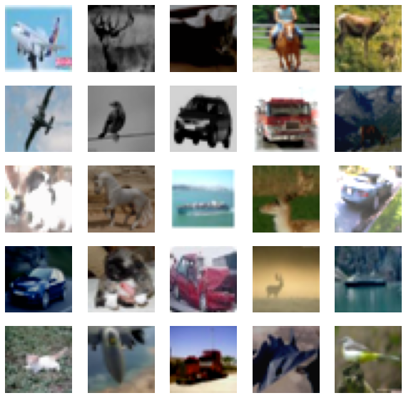
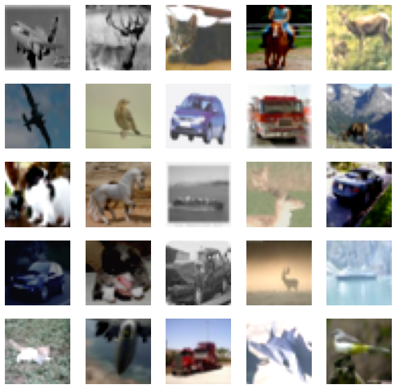
请注意,`samples_images_one` 和 `sample_images_two` 中的图像本质上是相同的,但经过了不同的增强。
定义编码器和预测器
我们使用了 ResNet20 的实现,该实现专门为 CIFAR10 数据集配置。代码摘自 keras-idiomatic-programmer 仓库。这些架构的超参数参考了 原始论文 的第 3 节和附录 A。
!wget -q https://git.io/JYx2x -O resnet_cifar10_v2.py
import resnet_cifar10_v2

N = 2
DEPTH = N * 9 + 2
NUM_BLOCKS = ((DEPTH - 2) // 9) - 1


def get_encoder():
    # Input and backbone.
    inputs = layers.Input((CROP_TO, CROP_TO, 3))
    x = layers.Rescaling(scale=1.0 / 127.5, offset=-1)(
        inputs
    )
    x = resnet_cifar10_v2.stem(x)
    x = resnet_cifar10_v2.learner(x, NUM_BLOCKS)
    x = layers.GlobalAveragePooling2D(name="backbone_pool")(x)

    # Projection head.
    x = layers.Dense(
        PROJECT_DIM, use_bias=False, kernel_regularizer=regularizers.l2(WEIGHT_DECAY)
    )(x)
    x = layers.BatchNormalization()(x)
    x = layers.ReLU()(x)
    x = layers.Dense(
        PROJECT_DIM, use_bias=False, kernel_regularizer=regularizers.l2(WEIGHT_DECAY)
    )(x)
    outputs = layers.BatchNormalization()(x)
    return keras.Model(inputs, outputs, name="encoder")


def get_predictor():
    model = keras.Sequential(
        [
            # Note the AutoEncoder-like structure.
            layers.Input((PROJECT_DIM,)),
            layers.Dense(
                LATENT_DIM,
                use_bias=False,
                kernel_regularizer=regularizers.l2(WEIGHT_DECAY),
            ),
            layers.ReLU(),
            layers.BatchNormalization(),
            layers.Dense(PROJECT_DIM),
        ],
        name="predictor",
    )
    return model
定义(预)训练循环
使用这类方法训练网络的主要原因之一是利用学习到的表征进行分类等下游任务。因此,这个特定的训练阶段也被称为预训练。
我们首先定义损失函数。
def compute_loss(p, z):
    # The authors of SimSiam emphasize the impact of
    # the `stop_gradient` operator in the paper as it
    # has an important role in the overall optimization.
    z = ops.stop_gradient(z)
    p = keras.utils.normalize(p, axis=1, order=2)
    z = keras.utils.normalize(z, axis=1, order=2)
    # Negative cosine similarity (minimizing this is
    # equivalent to maximizing the similarity).
    return -ops.mean(ops.sum((p * z), axis=1))
然后,我们通过重写 keras.Model 类的 train_step() 函数来定义我们的训练循环。
class SimSiam(keras.Model):
    def __init__(self, encoder, predictor):
        super().__init__()
        self.encoder = encoder
        self.predictor = predictor
        self.loss_tracker = keras.metrics.Mean(name="loss")

    @property
    def metrics(self):
        return [self.loss_tracker]

    def train_step(self, data):
        # Unpack the data.
        ds_one, ds_two = data

        # Forward pass through the encoder and predictor.
        with tf.GradientTape() as tape:
            z1, z2 = self.encoder(ds_one), self.encoder(ds_two)
            p1, p2 = self.predictor(z1), self.predictor(z2)
            # Note that here we are enforcing the network to match
            # the representations of two differently augmented batches
            # of data.
            loss = compute_loss(p1, z2) / 2 + compute_loss(p2, z1) / 2

        # Compute gradients and update the parameters.
        learnable_params = (
            self.encoder.trainable_variables + self.predictor.trainable_variables
        )
        gradients = tape.gradient(loss, learnable_params)
        self.optimizer.apply_gradients(zip(gradients, learnable_params))

        # Monitor loss.
        self.loss_tracker.update_state(loss)
        return {"loss": self.loss_tracker.result()}
预训练我们的网络
为了本示例的演示目的,我们将仅训练模型 5 个 epoch。实际上,这至少应该训练 100 个 epoch。
# Create a cosine decay learning scheduler.
num_training_samples = len(x_train)
steps = EPOCHS * (num_training_samples // BATCH_SIZE)
lr_decayed_fn = keras.optimizers.schedules.CosineDecay(
initial_learning_rate=0.03, decay_steps=steps
)
# Create an early stopping callback.
early_stopping = keras.callbacks.EarlyStopping(
monitor="loss", patience=5, restore_best_weights=True
)
# Compile model and start training.
simsiam = SimSiam(get_encoder(), get_predictor())
simsiam.compile(optimizer=keras.optimizers.SGD(lr_decayed_fn, momentum=0.6))
history = simsiam.fit(ssl_ds, epochs=EPOCHS, callbacks=[early_stopping])
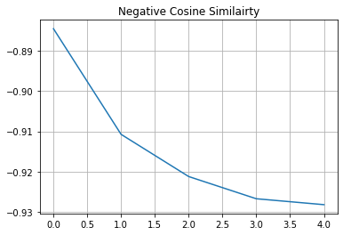
# Visualize the training progress of the model.
plt.plot(history.history["loss"])
plt.grid()
plt.title("Negative Cosine Similairty")
plt.show()
Epoch 1/5
391/391 [==============================] - 33s 42ms/step - loss: -0.8973
Epoch 2/5
391/391 [==============================] - 16s 40ms/step - loss: -0.9129
Epoch 3/5
391/391 [==============================] - 16s 40ms/step - loss: -0.9165
Epoch 4/5
391/391 [==============================] - 16s 40ms/step - loss: -0.9176
Epoch 5/5
391/391 [==============================] - 16s 40ms/step - loss: -0.9182
如果您的解决方案在不同的数据集和不同的骨干网络架构下,非常接近 -1(我们的损失函数的最小值),这很可能是由于表征坍塌。这是一种现象,即编码器会为所有图像产生相似的输出。在这种情况下,需要进行额外的超参数调整,尤其是在以下方面:
- 颜色失真的强度及其概率。
- 学习率及其调度。
- 骨干网络及其投影头的架构。
评估我们的 SSL 方法
评估计算机视觉领域 SSL 方法(或任何预训练方法)最常用的方法是在训练好的骨干模型(在本例中是 ResNet20)的冻结特征上学习一个线性分类器,并在未见过的数据上评估该分类器。其他方法包括在源数据集或具有 5% 或 10% 标签的目标数据集上进行微调。实践中,我们可以将骨干模型用于任何下游任务,如语义分割、目标检测等,而这些任务的骨干模型通常使用纯监督学习进行预训练。
# We first create labeled `Dataset` objects.
train_ds = tf.data.Dataset.from_tensor_slices((x_train, y_train))
test_ds = tf.data.Dataset.from_tensor_slices((x_test, y_test))

# Then we shuffle, batch, and prefetch this dataset for performance. We
# also apply random resized crops as an augmentation but only to the
# training set.
train_ds = (
    train_ds.shuffle(1024)
    .map(lambda x, y: (flip_random_crop(x), y), num_parallel_calls=AUTO)
    .batch(BATCH_SIZE)
    .prefetch(AUTO)
)
test_ds = test_ds.batch(BATCH_SIZE).prefetch(AUTO)

# Extract the backbone ResNet20.
backbone = keras.Model(
    simsiam.encoder.input, simsiam.encoder.get_layer("backbone_pool").output
)

# We then create our linear classifier and train it.
backbone.trainable = False
inputs = layers.Input((CROP_TO, CROP_TO, 3))
x = backbone(inputs, training=False)
outputs = layers.Dense(10, activation="softmax")(x)
linear_model = keras.Model(inputs, outputs, name="linear_model")

# Compile model and start training.
linear_model.compile(
    loss="sparse_categorical_crossentropy",
    metrics=["accuracy"],
    optimizer=keras.optimizers.SGD(lr_decayed_fn, momentum=0.9),
)
history = linear_model.fit(
    train_ds, validation_data=test_ds, epochs=EPOCHS, callbacks=[early_stopping]
)
_, test_acc = linear_model.evaluate(test_ds)
print("Test accuracy: {:.2f}%".format(test_acc * 100))
Epoch 1/5
391/391 [==============================] - 7s 11ms/step - loss: 3.8072 - accuracy: 0.1527 - val_loss: 3.7449 - val_accuracy: 0.2046
Epoch 2/5
391/391 [==============================] - 3s 8ms/step - loss: 3.7356 - accuracy: 0.2107 - val_loss: 3.7055 - val_accuracy: 0.2308
Epoch 3/5
391/391 [==============================] - 3s 8ms/step - loss: 3.7036 - accuracy: 0.2228 - val_loss: 3.6874 - val_accuracy: 0.2329
Epoch 4/5
391/391 [==============================] - 3s 8ms/step - loss: 3.6893 - accuracy: 0.2276 - val_loss: 3.6808 - val_accuracy: 0.2334
Epoch 5/5
391/391 [==============================] - 3s 9ms/step - loss: 3.6845 - accuracy: 0.2305 - val_loss: 3.6798 - val_accuracy: 0.2339
79/79 [==============================] - 1s 7ms/step - loss: 3.6798 - accuracy: 0.2339
Test accuracy: 23.39%