探究 Vision Transformer 的表示
作者: Aritra Roy Gosthipaty, Sayak Paul (贡献相同)
创建日期 2022/04/12
最后修改日期 2023/11/20
描述: 探究不同 Vision Transformer 变体的学习表示。

简介
在此示例中,我们探究了不同 Vision Transformer (ViT) 模型学习到的表示。此示例的主要目标是深入了解是什么使得 ViT 能够从图像数据中学习。特别是,该示例讨论了几个不同的 ViT 分析工具的实现。
注意: 当我们说“Vision Transformer”时,指的是一种包含 Transformer 块 (Vaswani 等人) 的计算机视觉架构,而不一定指原始的 Vision Transformer 模型 (Dosovitskiy 等人)。
考虑的模型
自原始 Vision Transformer 问世以来,计算机视觉领域出现了许多不同的 ViT 变体,它们在各种方面都优于原始模型:训练改进、架构改进等。在此示例中,我们考虑以下 ViT 模型系列
- 使用 ImageNet-1k 和 ImageNet-21k 数据集进行监督预训练的 ViT (Dosovitskiy 等人)
- 使用监督预训练但仅使用 ImageNet-1k 数据集进行训练,并带有更多正则化和蒸馏的 ViT (Touvron 等人) (DeiT)。
- 使用自监督预训练的 ViT (Caron 等人) (DINO)。
由于 Keras 中未实现预训练模型,我们首先尽可能忠实地实现了它们。然后,我们用官方的预训练参数填充了它们。最后,我们在 ImageNet-1k 验证集上评估了我们的实现,以确保评估数字与原始实现匹配。我们实现的详细信息可在 此存储库 中找到。
为了保持示例的简洁性,我们不会详尽地将每个模型与分析方法配对。我们将在相应的部分提供注释,以便您可以自行推导。
要在 Google Colab 上运行此示例,我们需要更新 gdown 库,如下所示
pip install -U gdown -q
导入
import os

os.environ["KERAS_BACKEND"] = "tensorflow"

import zipfile
from io import BytesIO

import cv2
import matplotlib.pyplot as plt
import numpy as np
import requests

from PIL import Image
from sklearn.preprocessing import MinMaxScaler
import keras
from keras import ops
常量
RESOLUTION = 224
PATCH_SIZE = 16
GITHUB_RELEASE = "https://github.com/sayakpaul/probing-vits/releases/download/v1.0.0/probing_vits.zip"
FNAME = "probing_vits.zip"
MODELS_ZIP = {
    "vit_dino_base16": "Probing_ViTs/vit_dino_base16.zip",
    "vit_b16_patch16_224": "Probing_ViTs/vit_b16_patch16_224.zip",
    "vit_b16_patch16_224-i1k_pretrained": "Probing_ViTs/vit_b16_patch16_224-i1k_pretrained.zip",
}
数据工具
对于原始 ViT 模型,输入图像需要缩放到 [-1, 1] 的范围。对于开头提到的其他模型系列,我们需要使用 ImageNet-1k 训练集的通道均值和标准差对图像进行归一化。
crop_layer = keras.layers.CenterCrop(RESOLUTION, RESOLUTION)
norm_layer = keras.layers.Normalization(
    mean=[0.485 * 255, 0.456 * 255, 0.406 * 255],
    variance=[(0.229 * 255) ** 2, (0.224 * 255) ** 2, (0.225 * 255) ** 2],
)
rescale_layer = keras.layers.Rescaling(scale=1.0 / 127.5, offset=-1)


def preprocess_image(image, model_type, size=RESOLUTION):
    # Turn the image into a numpy array and add batch dim.
    image = np.array(image)
    image = ops.expand_dims(image, 0)

    # If model type is vit rescale the image to [-1, 1].
    if model_type == "original_vit":
        image = rescale_layer(image)

    # Resize the image using bicubic interpolation.
    resize_size = int((256 / 224) * size)
    image = ops.image.resize(image, (resize_size, resize_size), interpolation="bicubic")

    # Crop the image.
    image = crop_layer(image)

    # If model type is DeiT or DINO normalize the image.
    if model_type != "original_vit":
        image = norm_layer(image)

    return ops.convert_to_numpy(image)


def load_image_from_url(url, model_type):
    # Credit: Willi Gierke
    response = requests.get(url)
    image = Image.open(BytesIO(response.content))
    preprocessed_image = preprocess_image(image, model_type)
    return image, preprocessed_image
加载测试图像并显示
# ImageNet-1k label mapping file and load it.
mapping_file = keras.utils.get_file(
origin="https://storage.googleapis.com/bit_models/ilsvrc2012_wordnet_lemmas.txt"
)
with open(mapping_file, "r") as f:
lines = f.readlines()
imagenet_int_to_str = [line.rstrip() for line in lines]
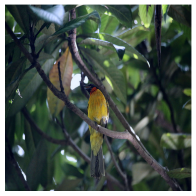
img_url = "https://dl.fbaipublicfiles.com/dino/img.png"
image, preprocessed_image = load_image_from_url(img_url, model_type="original_vit")
plt.imshow(image)
plt.axis("off")
plt.show()
加载模型
zip_path = keras.utils.get_file(
    fname=FNAME,
    origin=GITHUB_RELEASE,
)

with zipfile.ZipFile(zip_path, "r") as zip_ref:
    zip_ref.extractall("./")

os.rename("Probing ViTs", "Probing_ViTs")


def load_model(model_path: str) -> keras.Model:
    with zipfile.ZipFile(model_path, "r") as zip_ref:
        zip_ref.extractall("Probing_ViTs/")
    model_name = model_path.split(".")[0]

    inputs = keras.Input((RESOLUTION, RESOLUTION, 3))
    model = keras.layers.TFSMLayer(model_name, call_endpoint="serving_default")
    outputs = model(inputs, training=False)

    return keras.Model(inputs, outputs=outputs)


vit_base_i21k_patch16_224 = load_model(MODELS_ZIP["vit_b16_patch16_224-i1k_pretrained"])
print("Model loaded.")
Model loaded.
更多关于模型的信息:
该模型在 ImageNet-21k 数据集上进行了预训练,然后在 ImageNet-1k 数据集上进行了微调。要了解更多关于我们如何在 TensorFlow 中开发此模型(带有来自 此源 的预训练权重),请参考 此笔记本。
使用模型进行常规推理
我们现在对加载的模型在我们的测试图像上运行推理。
def split_prediction_and_attention_scores(outputs):
    predictions = outputs["output_1"]
    attention_score_dict = {}
    for key, value in outputs.items():
        if key.startswith("output_2_"):
            attention_score_dict[key[len("output_2_") :]] = value
    return predictions, attention_score_dict


predictions, attention_score_dict = split_prediction_and_attention_scores(
    vit_base_i21k_patch16_224.predict(preprocessed_image)
)
predicted_label = imagenet_int_to_str[int(np.argmax(predictions))]
print(predicted_label)
 1/1 ━━━━━━━━━━━━━━━━━━━━ 5s 5s/step
toucan

WARNING: All log messages before absl::InitializeLog() is called are written to STDERR
I0000 00:00:1700526824.965785   75784 device_compiler.h:187] Compiled cluster using XLA!  This line is logged at most once for the lifetime of the process.
attention_score_dict 包含每个 Transformer 块的每个注意力头的注意力分数(softmax 输出)。
方法一:平均注意力距离
Dosovitskiy 等人 和 Raghu 等人 使用一种称为“平均注意力距离”的度量,该度量从不同 Transformer 块的每个注意力头计算得出,以了解局部和全局信息如何流入 Vision Transformer。
平均注意力距离定义为查询 token 与其他 token 的距离乘以注意力权重。因此,对于单个图像
- 我们提取图像中的各个 patch(token),
- 计算它们的几何距离,然后
- 将其乘以注意力分数。
注意力分数是在通过网络进行推理模式前向传播后计算的。下图可能有助于您更好地理解该过程。

此动画由 Ritwik Raha 创建。
def compute_distance_matrix(patch_size, num_patches, length):
    distance_matrix = np.zeros((num_patches, num_patches))
    for i in range(num_patches):
        for j in range(num_patches):
            if i == j:  # zero distance
                continue

            xi, yi = (int(i / length)), (i % length)
            xj, yj = (int(j / length)), (j % length)
            distance_matrix[i, j] = patch_size * np.linalg.norm([xi - xj, yi - yj])

    return distance_matrix


def compute_mean_attention_dist(patch_size, attention_weights, model_type):
    num_cls_tokens = 2 if "distilled" in model_type else 1

    # The attention_weights shape = (batch, num_heads, num_patches, num_patches)
    attention_weights = attention_weights[
        ..., num_cls_tokens:, num_cls_tokens:
    ]  # Removing the CLS token
    num_patches = attention_weights.shape[-1]
    length = int(np.sqrt(num_patches))
    assert length**2 == num_patches, "Num patches is not perfect square"

    distance_matrix = compute_distance_matrix(patch_size, num_patches, length)
    h, w = distance_matrix.shape

    distance_matrix = distance_matrix.reshape((1, 1, h, w))
    # The attention_weights along the last axis adds to 1
    # this is due to the fact that they are softmax of the raw logits
    # summation of the (attention_weights * distance_matrix)
    # should result in an average distance per token.
    mean_distances = attention_weights * distance_matrix
    mean_distances = np.sum(
        mean_distances, axis=-1
    )  # Sum along last axis to get average distance per token
    mean_distances = np.mean(
        mean_distances, axis=-1
    )  # Now average across all the tokens

    return mean_distances
感谢 Google 的 Simon Kornblith,他为我们提供了此代码片段。您可以在 此处 找到它。现在,让我们使用这些工具来生成一个注意力距离与我们的加载模型和测试图像的图。
# Build the mean distances for every Transformer block.
mean_distances = {
    f"{name}_mean_dist": compute_mean_attention_dist(
        patch_size=PATCH_SIZE,
        attention_weights=attention_weight,
        model_type="original_vit",
    )
    for name, attention_weight in attention_score_dict.items()
}

# Get the number of heads from the mean distance output.
num_heads = mean_distances["transformer_block_0_att_mean_dist"].shape[-1]

# Print the shapes
print(f"Num Heads: {num_heads}.")

plt.figure(figsize=(9, 9))

for idx in range(len(mean_distances)):
    mean_distance = mean_distances[f"transformer_block_{idx}_att_mean_dist"]
    x = [idx] * num_heads
    y = mean_distance[0, :]
    plt.scatter(x=x, y=y, label=f"transformer_block_{idx}")

plt.legend(loc="lower right")
plt.xlabel("Attention Head", fontsize=14)
plt.ylabel("Attention Distance", fontsize=14)
plt.title("vit_base_i21k_patch16_224", fontsize=14)
plt.grid()
plt.show()
Num Heads: 12.
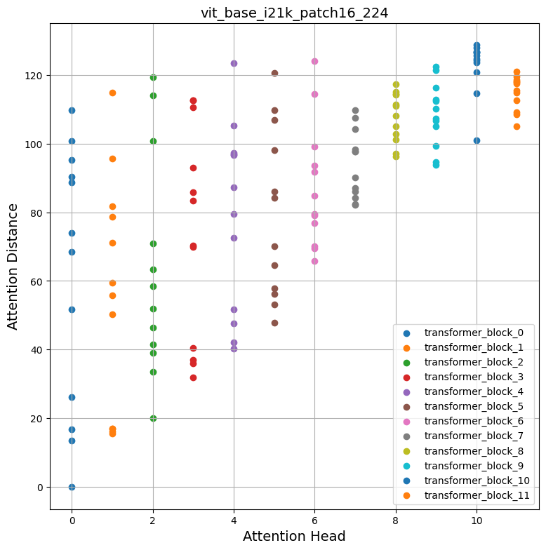
检查图表
自注意力如何在输入空间中跨越?它们关注输入区域是局部的还是全局的?
自注意力的承诺是能够学习上下文依赖关系,以便模型可以关注输入中最与目标相关的区域。从上面的图中,我们可以注意到不同的注意力头产生不同的注意力距离,这表明它们同时利用图像中的局部和全局信息。但是,当我们深入 Transformer 块时,注意力头倾向于更多地关注全局聚合信息。
受 Raghu 等人 的启发,我们计算了从 ImageNet-1k 验证集中随机选择的 1000 张图像的平均注意力距离,并对开头提到的所有模型重复了该过程。有趣的是,我们注意到以下几点
- 使用更大的数据集进行预训练有助于更长的全局注意力跨度
| 在 ImageNet-21k 上预训练 在 ImageNet-1k 上微调 |
在 ImageNet-1k 上预训练 |
|---|---|
- 当从 CNN 蒸馏时,ViT 倾向于具有更短的全局注意力跨度
| 无蒸馏 (DeiT 的 ViT B-16) | DeiT 的蒸馏 ViT B-16 |
|---|---|
要重现这些图表,请参考 此笔记本。
方法二:注意力展开 (Attention Rollout)
Abnar 等人 引入了“注意力展开”来量化信息如何通过 Transformer 块的自注意力层流动。原始 ViT 作者使用此方法来研究学习到的表示,并指出
简而言之,我们对 ViTL/16 在所有注意力头上的注意力权重进行了平均,然后递归地将所有层的权重矩阵相乘。这考虑了跨 token 的注意力在所有层中的混合。
我们使用了 此笔记本 并修改了其中的注意力展开代码,以兼容我们的模型。
def attention_rollout_map(image, attention_score_dict, model_type):
    num_cls_tokens = 2 if "distilled" in model_type else 1

    # Stack the individual attention matrices from individual Transformer blocks.
    attn_mat = ops.stack([attention_score_dict[k] for k in attention_score_dict.keys()])
    attn_mat = ops.squeeze(attn_mat, axis=1)

    # Average the attention weights across all heads.
    attn_mat = ops.mean(attn_mat, axis=1)

    # To account for residual connections, we add an identity matrix to the
    # attention matrix and re-normalize the weights.
    residual_attn = ops.eye(attn_mat.shape[1])
    aug_attn_mat = attn_mat + residual_attn
    aug_attn_mat = aug_attn_mat / ops.sum(aug_attn_mat, axis=-1)[..., None]
    aug_attn_mat = ops.convert_to_numpy(aug_attn_mat)

    # Recursively multiply the weight matrices.
    joint_attentions = np.zeros(aug_attn_mat.shape)
    joint_attentions[0] = aug_attn_mat[0]

    for n in range(1, aug_attn_mat.shape[0]):
        joint_attentions[n] = np.matmul(aug_attn_mat[n], joint_attentions[n - 1])

    # Attention from the output token to the input space.
    v = joint_attentions[-1]
    grid_size = int(np.sqrt(aug_attn_mat.shape[-1]))
    mask = v[0, num_cls_tokens:].reshape(grid_size, grid_size)
    mask = cv2.resize(mask / mask.max(), image.size)[..., np.newaxis]
    result = (mask * image).astype("uint8")
    return result
现在,让我们使用这些工具根据我们之前在“使用模型进行常规推理”部分的结果生成一张注意力图。以下是下载每个单独模型的链接
- 原始 ViT 模型(在 ImageNet-21k 上预训练)
- 原始 ViT 模型(在 ImageNet-1k 上预训练)
- DINO 模型(在 ImageNet-1k 上预训练)
- DeiT 模型(在 ImageNet-1k 上预训练,包括蒸馏和非蒸馏模型)
attn_rollout_result = attention_rollout_map(
    image, attention_score_dict, model_type="original_vit"
)

fig, (ax1, ax2) = plt.subplots(ncols=2, figsize=(8, 10))
fig.suptitle(f"Predicted label: {predicted_label}.", fontsize=20)

_ = ax1.imshow(image)
_ = ax2.imshow(attn_rollout_result)
ax1.set_title("Input Image", fontsize=16)
ax2.set_title("Attention Map", fontsize=16)
ax1.axis("off")
ax2.axis("off")

fig.tight_layout()
fig.subplots_adjust(top=1.35)
fig.show()
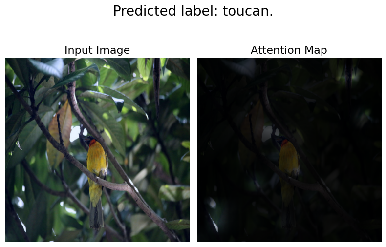
检查图表
我们如何量化通过注意力层传播的信息流?
我们注意到模型能够将其注意力集中在输入图像的重要部分。我们鼓励您将此方法应用于我们提到的其他模型,并比较结果。注意力展开图将根据模型训练的任务和增强方式而有所不同。我们观察到 DeiT 具有最佳的展开图,这可能是由于其增强策略。
方法三:注意力热图
探究 Vision Transformer 表示的一种简单但有用的方法是将注意力图叠加在输入图像上进行可视化。这有助于形成关于模型关注内容的直观认识。我们为此目的使用了 DINO 模型,因为它能产生更好的注意力热图。
# Load the model.
vit_dino_base16 = load_model(MODELS_ZIP["vit_dino_base16"])
print("Model loaded.")

# Preprocess the same image but with normlization.
img_url = "https://dl.fbaipublicfiles.com/dino/img.png"
image, preprocessed_image = load_image_from_url(img_url, model_type="dino")

# Grab the predictions.
predictions, attention_score_dict = split_prediction_and_attention_scores(
    vit_dino_base16.predict(preprocessed_image)
)
Model loaded.
 1/1 ━━━━━━━━━━━━━━━━━━━━ 4s 4s/step
一个 Transformer 块包含多个头。Transformer 块中的每个头将输入数据投影到不同的子空间。这有助于每个单独的头关注图像的不同部分。因此,有必要单独可视化每个注意力头图,以便理解每个头关注的内容。
注意事项:
- 下面的代码是从 原始 DINO 代码库 复制修改的。
- 在这里,我们提取最后一个 Transformer 块的注意力图。
- DINO 使用自监督目标进行了预训练。
def attention_heatmap(attention_score_dict, image, model_type="dino"):
    num_tokens = 2 if "distilled" in model_type else 1

    # Sort the Transformer blocks in order of their depth.
    attention_score_list = list(attention_score_dict.keys())
    attention_score_list.sort(key=lambda x: int(x.split("_")[-2]), reverse=True)

    # Process the attention maps for overlay.
    w_featmap = image.shape[2] // PATCH_SIZE
    h_featmap = image.shape[1] // PATCH_SIZE
    attention_scores = attention_score_dict[attention_score_list[0]]

    # Taking the representations from CLS token.
    attentions = attention_scores[0, :, 0, num_tokens:].reshape(num_heads, -1)

    # Reshape the attention scores to resemble mini patches.
    attentions = attentions.reshape(num_heads, w_featmap, h_featmap)
    attentions = attentions.transpose((1, 2, 0))

    # Resize the attention patches to 224x224 (224: 14x16).
    attentions = ops.image.resize(
        attentions, size=(h_featmap * PATCH_SIZE, w_featmap * PATCH_SIZE)
    )
    return attentions
我们可以使用与 DINO 推理相同的图像以及我们从结果中提取的 attention_score_dict。
# De-normalize the image for visual clarity.
in1k_mean = np.array([0.485 * 255, 0.456 * 255, 0.406 * 255])
in1k_std = np.array([0.229 * 255, 0.224 * 255, 0.225 * 255])
preprocessed_img_orig = (preprocessed_image * in1k_std) + in1k_mean
preprocessed_img_orig = preprocessed_img_orig / 255.0
preprocessed_img_orig = ops.convert_to_numpy(ops.clip(preprocessed_img_orig, 0.0, 1.0))

# Generate the attention heatmaps.
attentions = attention_heatmap(attention_score_dict, preprocessed_img_orig)

# Plot the maps.
fig, axes = plt.subplots(nrows=3, ncols=4, figsize=(13, 13))
img_count = 0

for i in range(3):
    for j in range(4):
        if img_count < len(attentions):
            axes[i, j].imshow(preprocessed_img_orig[0])
            axes[i, j].imshow(attentions[..., img_count], cmap="inferno", alpha=0.6)
            axes[i, j].title.set_text(f"Attention head: {img_count}")
            axes[i, j].axis("off")
            img_count += 1
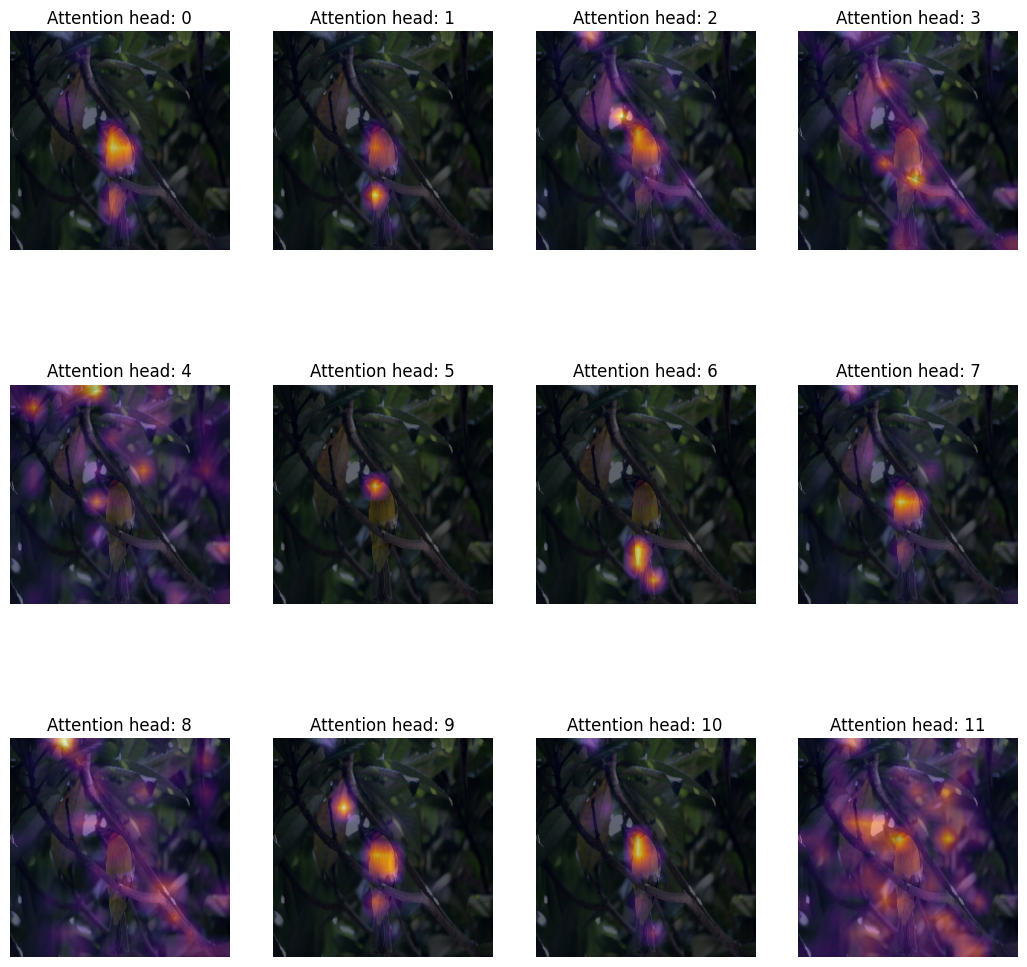
检查图表
我们如何定性评估注意力权重?
Transformer 块的注意力权重是在键(key)和查询(query)之间计算的。权重量化了键对查询的重要性。在 ViT 中,键和查询来自同一图像,因此权重决定了图像的哪个部分很重要。
将注意力权重叠加在图像上进行绘制,可以让我们对 Transformer 重要的图像部分产生直观认识。此图定性地评估了注意力权重的用途。
方法四:可视化学习到的投影滤波器
在提取不重叠的 patch 后,ViT 会将这些 patch 沿着其空间维度展平,然后进行线性投影。人们可能会想,这些投影看起来像什么?下面,我们以 ViT B-16 模型为例,可视化其学习到的投影。
def extract_weights(model, name):
    for variable in model.weights:
        if variable.name.startswith(name):
            return variable.numpy()


# Extract the projections.
projections = extract_weights(vit_base_i21k_patch16_224, "conv_projection/kernel")
projection_dim = projections.shape[-1]
patch_h, patch_w, patch_channels = projections.shape[:-1]

# Scale the projections.
scaled_projections = MinMaxScaler().fit_transform(
    projections.reshape(-1, projection_dim)
)

# Reshape the scaled projections so that the leading
# three dimensions resemble an image.
scaled_projections = scaled_projections.reshape(patch_h, patch_w, patch_channels, -1)

# Visualize the first 128 filters of the learned
# projections.
fig, axes = plt.subplots(nrows=8, ncols=16, figsize=(13, 8))
img_count = 0
limit = 128

for i in range(8):
    for j in range(16):
        if img_count < limit:
            axes[i, j].imshow(scaled_projections[..., img_count])
            axes[i, j].axis("off")
            img_count += 1

fig.tight_layout()
WARNING:matplotlib.image:Clipping input data to the valid range for imshow with RGB data ([0..1] for floats or [0..255] for integers).
WARNING:matplotlib.image:Clipping input data to the valid range for imshow with RGB data ([0..1] for floats or [0..255] for integers).
WARNING:matplotlib.image:Clipping input data to the valid range for imshow with RGB data ([0..1] for floats or [0..255] for integers).
WARNING:matplotlib.image:Clipping input data to the valid range for imshow with RGB data ([0..1] for floats or [0..255] for integers).
WARNING:matplotlib.image:Clipping input data to the valid range for imshow with RGB data ([0..1] for floats or [0..255] for integers).
WARNING:matplotlib.image:Clipping input data to the valid range for imshow with RGB data ([0..1] for floats or [0..255] for integers).
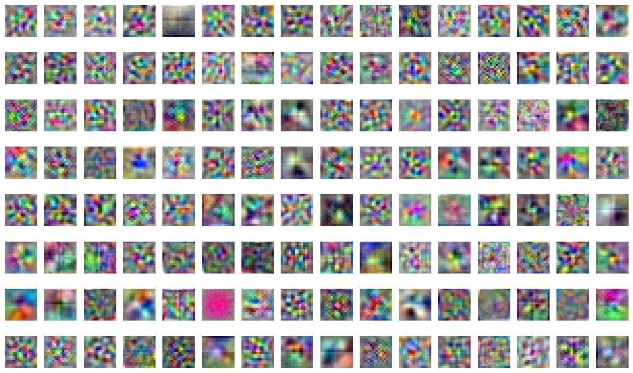
检查图表
投影滤波器学习了什么?
可视化时,卷积神经网络的核显示了它们在图像中寻找的模式。这可能是圆圈,有时是线条——当它们组合在一起时(在卷积网络的后期),滤波器会变成更复杂的形状。我们发现这些卷积核与 ViT 的投影滤波器之间存在明显相似性。
方法五:可视化位置嵌入
Transformer 对排列是不变的。这意味着它们不考虑输入 token 的空间位置。为了克服这个限制,我们向输入 token 添加了位置信息。
位置信息可以是学习到的位置嵌入或手工制作的常量嵌入。在我们的例子中,ViT 的所有三个变体都具有学习到的位置嵌入。
在本节中,我们可视化了学习到的位置嵌入与其自身的相似性。下面,我们以 ViT B-16 模型为例,通过取其点积来可视化位置嵌入的相似性。
position_embeddings = extract_weights(vit_base_i21k_patch16_224, "pos_embedding")

# Discard the batch dimension and the position embeddings of the
# cls token.
position_embeddings = position_embeddings.squeeze()[1:, ...]

similarity = position_embeddings @ position_embeddings.T
plt.imshow(similarity, cmap="inferno")
plt.show()
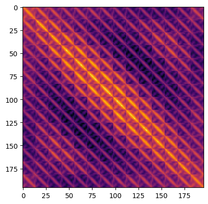
检查图表
位置嵌入告诉我们什么?
该图具有独特的对角线图案。主对角线最亮,表示一个位置与自身最相似。一个有趣的模式是重复的对角线。重复的模式描绘了一个正弦函数,这与 Vaswani 等人 提出的手工制作特征非常接近。
注意事项
-
DINO 将注意力热图生成过程扩展到了视频。我们还 将 我们的 DINO 实现应用于一系列视频,并获得了类似的结果。这是一个注意力热图的视频

- Raghu 等人 使用一系列技术来探究 ViT 学习到的表示,并将其与 ResNets 进行比较。我们强烈建议阅读他们的工作。
- 为了编写这个示例,我们开发了 此存储库 来指导我们的读者,以便他们可以轻松地重现实验并进行扩展。
- 另一个您可能会对此感兴趣的存储库是
vit-explain。
- 您也可以使用我们的 Hugging Face Spaces,用自定义图像绘制注意力展开图和注意力热图。
| 注意力热图 | 注意力展开 |
|---|---|