PointNet 点云分割
作者: Soumik Rakshit, Sayak Paul
创建日期 2020/10/23
最后修改日期 2020/10/24
描述: 实现基于 PointNet 的点云分割模型。

简介
“点云”是存储几何形状数据的重要数据结构。由于其格式不规则,在用于深度学习应用之前,通常会将其转换为规则的 3D 体素网格或图像集合,这一步骤会使数据变得不必要地庞大。PointNet 系列模型通过直接处理点云来解决这个问题,尊重点数据的排列不变性。PointNet 系列模型为从 **物体分类**、**部件分割** 到 **场景语义解析** 的应用提供了一个简单、统一的架构。
在本例中,我们演示了 PointNet 架构在形状分割中的实现。
参考文献
导入
import os
import json
import random
import numpy as np
import pandas as pd
from tqdm import tqdm
from glob import glob

import tensorflow as tf  # For tf.data
import keras
from keras import layers

import matplotlib.pyplot as plt
下载数据集
ShapeNet 数据集 是一个持续的努力,旨在建立一个丰富标注、大规模的 3D 模型数据集。**ShapeNetCore** 是完整 ShapeNet 数据集的一个子集,其中包含干净的单个 3D 模型和手动验证的类别及对齐标注。它涵盖了 55 个常见物体类别,约有 51,300 个独特的 3D 模型。
在本例中,我们使用了 PASCAL 3D+ 数据集中的 12 个物体类别之一,该类别也包含在 ShapenetCore 数据集中。
dataset_url = "https://git.io/JiY4i"

dataset_path = keras.utils.get_file(
    fname="shapenet.zip",
    origin=dataset_url,
    cache_subdir="datasets",
    hash_algorithm="auto",
    extract=True,
    archive_format="auto",
    cache_dir="datasets",
)
加载数据集
我们解析数据集元数据,以便轻松地将模型类别映射到其对应的目录,并将分割类别映射到颜色,以便于可视化。
with open("/tmp/.keras/datasets/PartAnnotation/metadata.json") as json_file:
    metadata = json.load(json_file)

print(metadata)
{'Airplane': {'directory': '02691156', 'lables': ['wing', 'body', 'tail', 'engine'], 'colors': ['blue', 'green', 'red', 'pink']}, 'Bag': {'directory': '02773838', 'lables': ['handle', 'body'], 'colors': ['blue', 'green']}, 'Cap': {'directory': '02954340', 'lables': ['panels', 'peak'], 'colors': ['blue', 'green']}, 'Car': {'directory': '02958343', 'lables': ['wheel', 'hood', 'roof'], 'colors': ['blue', 'green', 'red']}, 'Chair': {'directory': '03001627', 'lables': ['leg', 'arm', 'back', 'seat'], 'colors': ['blue', 'green', 'red', 'pink']}, 'Earphone': {'directory': '03261776', 'lables': ['earphone', 'headband'], 'colors': ['blue', 'green']}, 'Guitar': {'directory': '03467517', 'lables': ['head', 'body', 'neck'], 'colors': ['blue', 'green', 'red']}, 'Knife': {'directory': '03624134', 'lables': ['handle', 'blade'], 'colors': ['blue', 'green']}, 'Lamp': {'directory': '03636649', 'lables': ['canopy', 'lampshade', 'base'], 'colors': ['blue', 'green', 'red']}, 'Laptop': {'directory': '03642806', 'lables': ['keyboard'], 'colors': ['blue']}, 'Motorbike': {'directory': '03790512', 'lables': ['wheel', 'handle', 'gas_tank', 'light', 'seat'], 'colors': ['blue', 'green', 'red', 'pink', 'yellow']}, 'Mug': {'directory': '03797390', 'lables': ['handle'], 'colors': ['blue']}, 'Pistol': {'directory': '03948459', 'lables': ['trigger_and_guard', 'handle', 'barrel'], 'colors': ['blue', 'green', 'red']}, 'Rocket': {'directory': '04099429', 'lables': ['nose', 'body', 'fin'], 'colors': ['blue', 'green', 'red']}, 'Skateboard': {'directory': '04225987', 'lables': ['wheel', 'deck'], 'colors': ['blue', 'green']}, 'Table': {'directory': '04379243', 'lables': ['leg', 'top'], 'colors': ['blue', 'green']}}
在本例中,我们训练 PointNet 来分割“飞机”模型的各个部件。
points_dir = "/tmp/.keras/datasets/PartAnnotation/{}/points".format(
    metadata["Airplane"]["directory"]
)
labels_dir = "/tmp/.keras/datasets/PartAnnotation/{}/points_label".format(
    metadata["Airplane"]["directory"]
)
LABELS = metadata["Airplane"]["lables"]
COLORS = metadata["Airplane"]["colors"]

VAL_SPLIT = 0.2
NUM_SAMPLE_POINTS = 1024
BATCH_SIZE = 32
EPOCHS = 60
INITIAL_LR = 1e-3
组织数据集结构
我们从飞机点云及其标签生成以下内存数据结构:
point_clouds是一个 `np.array` 对象列表,表示点云数据,格式为 x、y 和 z 坐标。轴 0 表示点云中的点数,轴 1 表示坐标。all_labels是表示每个坐标的标签(主要是为了可视化)的字符串列表。test_point_clouds的格式与point_clouds相同,但没有对应的点云标签。all_labels是一个 `np.array` 对象列表,表示每个坐标的点云标签,对应于point_clouds列表。point_cloud_labels是一个 `np.array` 对象列表,表示每个坐标的点云标签,以 one-hot 编码形式呈现,对应于point_clouds列表。
point_clouds, test_point_clouds = [], []
point_cloud_labels, all_labels = [], []

points_files = glob(os.path.join(points_dir, "*.pts"))
for point_file in tqdm(points_files):
    point_cloud = np.loadtxt(point_file)
    if point_cloud.shape[0] < NUM_SAMPLE_POINTS:
        continue

    # Get the file-id of the current point cloud for parsing its
    # labels.
    file_id = point_file.split("/")[-1].split(".")[0]
    label_data, num_labels = {}, 0
    for label in LABELS:
        label_file = os.path.join(labels_dir, label, file_id + ".seg")
        if os.path.exists(label_file):
            label_data[label] = np.loadtxt(label_file).astype("float32")
            num_labels = len(label_data[label])

    # Point clouds having labels will be our training samples.
    try:
        label_map = ["none"] * num_labels
        for label in LABELS:
            for i, data in enumerate(label_data[label]):
                label_map[i] = label if data == 1 else label_map[i]
        label_data = [
            LABELS.index(label) if label != "none" else len(LABELS)
            for label in label_map
        ]
        # Apply one-hot encoding to the dense label representation.
        label_data = keras.utils.to_categorical(label_data, num_classes=len(LABELS) + 1)

        point_clouds.append(point_cloud)
        point_cloud_labels.append(label_data)
        all_labels.append(label_map)
    except KeyError:
        test_point_clouds.append(point_cloud)
100%|██████████████████████████████████████████████████████████████████████| 4045/4045 [01:30<00:00, 44.54it/s]
接下来,我们看一些刚生成的内存数组中的样本。
for _ in range(5):
    i = random.randint(0, len(point_clouds) - 1)
    print(f"point_clouds[{i}].shape:", point_clouds[0].shape)
    print(f"point_cloud_labels[{i}].shape:", point_cloud_labels[0].shape)
    for j in range(5):
        print(
            f"all_labels[{i}][{j}]:",
            all_labels[i][j],
            f"\tpoint_cloud_labels[{i}][{j}]:",
            point_cloud_labels[i][j],
            "\n",
        )
point_clouds[333].shape: (2571, 3)
point_cloud_labels[333].shape: (2571, 5)
all_labels[333][0]: tail    point_cloud_labels[333][0]: [0. 0. 1. 0. 0.]
all_labels[333][1]: wing point_cloud_labels[333][1]: [1. 0. 0. 0. 0.]
all_labels[333][2]: tail point_cloud_labels[333][2]: [0. 0. 1. 0. 0.]
all_labels[333][3]: engine point_cloud_labels[333][3]: [0. 0. 0. 1. 0.]
all_labels[333][4]: wing point_cloud_labels[333][4]: [1. 0. 0. 0. 0.]
point_clouds[3273].shape: (2571, 3)
point_cloud_labels[3273].shape: (2571, 5)
all_labels[3273][0]: body   point_cloud_labels[3273][0]: [0. 1. 0. 0. 0.]
all_labels[3273][1]: body point_cloud_labels[3273][1]: [0. 1. 0. 0. 0.]
all_labels[3273][2]: tail point_cloud_labels[3273][2]: [0. 0. 1. 0. 0.]
all_labels[3273][3]: wing point_cloud_labels[3273][3]: [1. 0. 0. 0. 0.]
all_labels[3273][4]: wing point_cloud_labels[3273][4]: [1. 0. 0. 0. 0.]
point_clouds[929].shape: (2571, 3)
point_cloud_labels[929].shape: (2571, 5)
all_labels[929][0]: body    point_cloud_labels[929][0]: [0. 1. 0. 0. 0.]
all_labels[929][1]: tail point_cloud_labels[929][1]: [0. 0. 1. 0. 0.]
all_labels[929][2]: wing point_cloud_labels[929][2]: [1. 0. 0. 0. 0.]
all_labels[929][3]: tail point_cloud_labels[929][3]: [0. 0. 1. 0. 0.]
all_labels[929][4]: body point_cloud_labels[929][4]: [0. 1. 0. 0. 0.]
point_clouds[496].shape: (2571, 3)
point_cloud_labels[496].shape: (2571, 5)
all_labels[496][0]: body    point_cloud_labels[496][0]: [0. 1. 0. 0. 0.]
all_labels[496][1]: body point_cloud_labels[496][1]: [0. 1. 0. 0. 0.]
all_labels[496][2]: body point_cloud_labels[496][2]: [0. 1. 0. 0. 0.]
all_labels[496][3]: wing point_cloud_labels[496][3]: [1. 0. 0. 0. 0.]
all_labels[496][4]: body point_cloud_labels[496][4]: [0. 1. 0. 0. 0.]
point_clouds[3508].shape: (2571, 3)
point_cloud_labels[3508].shape: (2571, 5)
all_labels[3508][0]: body   point_cloud_labels[3508][0]: [0. 1. 0. 0. 0.]
all_labels[3508][1]: body point_cloud_labels[3508][1]: [0. 1. 0. 0. 0.]
all_labels[3508][2]: body point_cloud_labels[3508][2]: [0. 1. 0. 0. 0.]
all_labels[3508][3]: body point_cloud_labels[3508][3]: [0. 1. 0. 0. 0.]
all_labels[3508][4]: body point_cloud_labels[3508][4]: [0. 1. 0. 0. 0.]
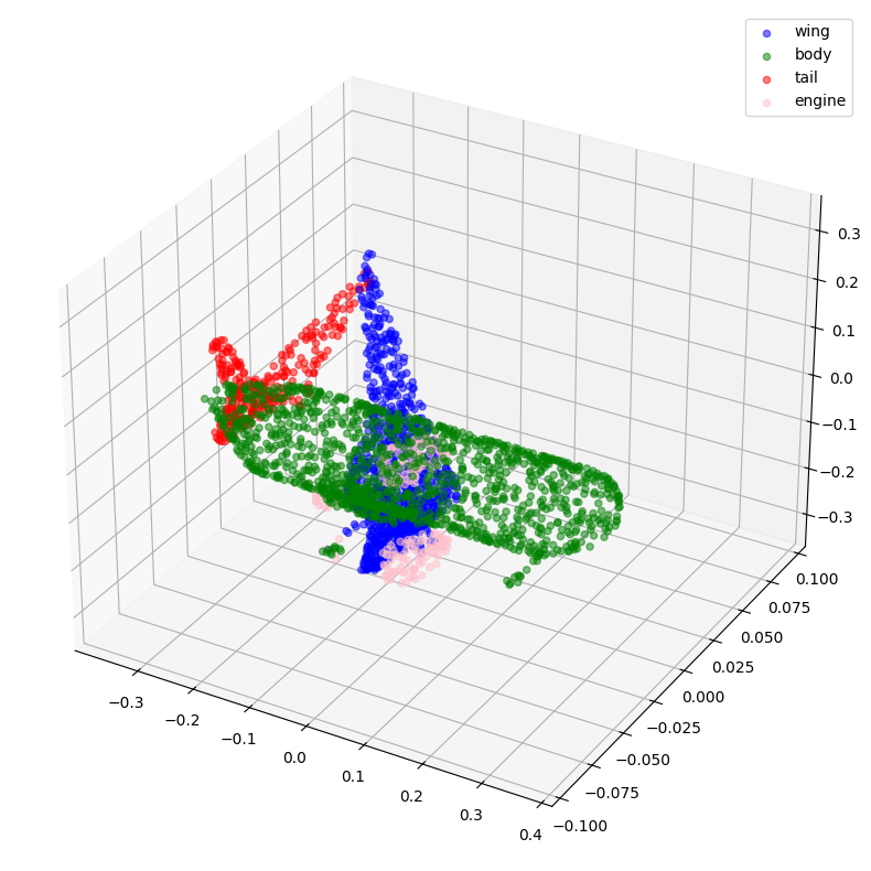
现在,让我们可视化一些点云及其标签。
def visualize_data(point_cloud, labels):
    df = pd.DataFrame(
        data={
            "x": point_cloud[:, 0],
            "y": point_cloud[:, 1],
            "z": point_cloud[:, 2],
            "label": labels,
        }
    )
    fig = plt.figure(figsize=(15, 10))
    ax = plt.axes(projection="3d")
    for index, label in enumerate(LABELS):
        c_df = df[df["label"] == label]
        try:
            ax.scatter(
                c_df["x"], c_df["y"], c_df["z"], label=label, alpha=0.5, c=COLORS[index]
            )
        except IndexError:
            pass
    ax.legend()
    plt.show()


visualize_data(point_clouds[0], all_labels[0])
visualize_data(point_clouds[300], all_labels[300])
预处理
请注意,我们加载的所有点云都包含可变数量的点,这使得我们难以将它们批量处理。为了解决这个问题,我们从每个点云中随机采样固定数量的点。我们还对点云进行归一化,以使数据具有尺度不变性。
for index in tqdm(range(len(point_clouds))):
    current_point_cloud = point_clouds[index]
    current_label_cloud = point_cloud_labels[index]
    current_labels = all_labels[index]
    num_points = len(current_point_cloud)
    # Randomly sampling respective indices.
    sampled_indices = random.sample(list(range(num_points)), NUM_SAMPLE_POINTS)
    # Sampling points corresponding to sampled indices.
    sampled_point_cloud = np.array([current_point_cloud[i] for i in sampled_indices])
    # Sampling corresponding one-hot encoded labels.
    sampled_label_cloud = np.array([current_label_cloud[i] for i in sampled_indices])
    # Sampling corresponding labels for visualization.
    sampled_labels = np.array([current_labels[i] for i in sampled_indices])
    # Normalizing sampled point cloud.
    norm_point_cloud = sampled_point_cloud - np.mean(sampled_point_cloud, axis=0)
    norm_point_cloud /= np.max(np.linalg.norm(norm_point_cloud, axis=1))
    point_clouds[index] = norm_point_cloud
    point_cloud_labels[index] = sampled_label_cloud
    all_labels[index] = sampled_labels
100%|█████████████████████████████████████████████████████████████████████| 3694/3694 [00:08<00:00, 446.45it/s]
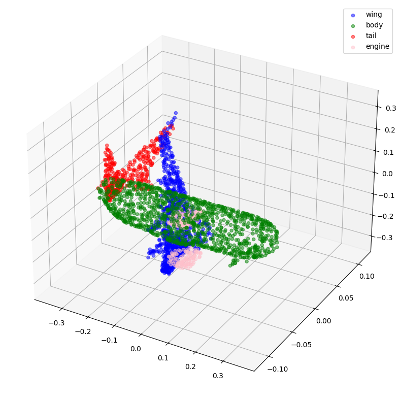
让我们可视化采样和归一化后的点云及其对应的标签。
visualize_data(point_clouds[0], all_labels[0])
visualize_data(point_clouds[300], all_labels[300])

创建 TensorFlow 数据集
我们为训练和验证数据创建 tf.data.Dataset 对象。我们还通过对训练点云应用随机抖动来对其进行增强。
def load_data(point_cloud_batch, label_cloud_batch):
    point_cloud_batch.set_shape([NUM_SAMPLE_POINTS, 3])
    label_cloud_batch.set_shape([NUM_SAMPLE_POINTS, len(LABELS) + 1])
    return point_cloud_batch, label_cloud_batch


def augment(point_cloud_batch, label_cloud_batch):
    noise = tf.random.uniform(
        tf.shape(label_cloud_batch), -0.001, 0.001, dtype=tf.float64
    )
    point_cloud_batch += noise[:, :, :3]
    return point_cloud_batch, label_cloud_batch


def generate_dataset(point_clouds, label_clouds, is_training=True):
    dataset = tf.data.Dataset.from_tensor_slices((point_clouds, label_clouds))
    dataset = dataset.shuffle(BATCH_SIZE * 100) if is_training else dataset
    dataset = dataset.map(load_data, num_parallel_calls=tf.data.AUTOTUNE)
    dataset = dataset.batch(batch_size=BATCH_SIZE)
    dataset = (
        dataset.map(augment, num_parallel_calls=tf.data.AUTOTUNE)
        if is_training
        else dataset
    )
    return dataset


split_index = int(len(point_clouds) * (1 - VAL_SPLIT))
train_point_clouds = point_clouds[:split_index]
train_label_cloud = point_cloud_labels[:split_index]
total_training_examples = len(train_point_clouds)

val_point_clouds = point_clouds[split_index:]
val_label_cloud = point_cloud_labels[split_index:]

print("Num train point clouds:", len(train_point_clouds))
print("Num train point cloud labels:", len(train_label_cloud))
print("Num val point clouds:", len(val_point_clouds))
print("Num val point cloud labels:", len(val_label_cloud))

train_dataset = generate_dataset(train_point_clouds, train_label_cloud)
val_dataset = generate_dataset(val_point_clouds, val_label_cloud, is_training=False)

print("Train Dataset:", train_dataset)
print("Validation Dataset:", val_dataset)
Num train point clouds: 2955
Num train point cloud labels: 2955
Num val point clouds: 739
Num val point cloud labels: 739
Train Dataset: <_ParallelMapDataset element_spec=(TensorSpec(shape=(None, 1024, 3), dtype=tf.float64, name=None), TensorSpec(shape=(None, 1024, 5), dtype=tf.float64, name=None))>
Validation Dataset: <_BatchDataset element_spec=(TensorSpec(shape=(None, 1024, 3), dtype=tf.float64, name=None), TensorSpec(shape=(None, 1024, 5), dtype=tf.float64, name=None))>
PointNet 模型
下图描绘了 PointNet 模型系列的内部结构。

鉴于 PointNet 的设计目的是处理 **无序点集** 作为输入数据,其架构需要匹配点云数据的以下特性:
排列不变性
鉴于点云数据的非结构化性质,由 `n` 个点组成的扫描有 `n!` 种排列。后续的数据处理必须对不同的表示具有不变性。为了使 PointNet 对输入排列具有不变性,我们在将 `n` 个输入点映射到更高维空间后,使用对称函数(如最大池化)。结果是一个 **全局特征向量**,旨在捕获 `n` 个输入点的聚合签名。全局特征向量与局部点特征一起用于分割。

变换不变性
如果物体经历某些变换(如平移或缩放),分割输出应保持不变。对于给定的输入点云,我们应用适当的刚性或仿射变换来实现姿态归一化。由于 `n` 个输入点中的每个点都表示为一个向量,并独立地映射到嵌入空间,应用几何变换仅仅相当于用变换矩阵对每个点进行矩阵乘法。这受到 空间变换网络 概念的启发。
T-Net 所包含的操作受到 PointNet 更高层架构的启发。MLP(或全连接层)用于将输入点独立且相同地映射到更高维空间;最大池化用于编码全局特征向量,然后使用全连接层减小其维度。最后全连接层的输入相关特征与全局可训练的权重和偏置相结合,生成一个 3x3 的变换矩阵。

点交互
相邻点之间的交互通常携带有用信息(即,单个点不应被孤立对待)。虽然分类只需要利用全局特征,但分割必须能够利用局部点特征以及全局点特征。
注意:本节中显示的图取自 原始论文。
现在我们了解了 PointNet 模型组成的各个部分,就可以实现该模型了。我们首先实现基本块,即卷积块和多层感知器块。
def conv_block(x, filters, name):
    x = layers.Conv1D(filters, kernel_size=1, padding="valid", name=f"{name}_conv")(x)
    x = layers.BatchNormalization(name=f"{name}_batch_norm")(x)
    return layers.Activation("relu", name=f"{name}_relu")(x)


def mlp_block(x, filters, name):
    x = layers.Dense(filters, name=f"{name}_dense")(x)
    x = layers.BatchNormalization(name=f"{name}_batch_norm")(x)
    return layers.Activation("relu", name=f"{name}_relu")(x)
我们实现了一个正则化器(取自 此示例),以强制特征空间的正交性。这对于确保变换后特征的幅度不会变化太大至关重要。
class OrthogonalRegularizer(keras.regularizers.Regularizer):
    """Reference: https://keras.org.cn/examples/vision/pointnet/#build-a-model"""

    def __init__(self, num_features, l2reg=0.001):
        self.num_features = num_features
        self.l2reg = l2reg
        self.identity = keras.ops.eye(num_features)

    def __call__(self, x):
        x = keras.ops.reshape(x, (-1, self.num_features, self.num_features))
        xxt = keras.ops.tensordot(x, x, axes=(2, 2))
        xxt = keras.ops.reshape(xxt, (-1, self.num_features, self.num_features))
        return keras.ops.sum(self.l2reg * keras.ops.square(xxt - self.identity))

    def get_config(self):
        config = super().get_config()
        config.update({"num_features": self.num_features, "l2reg_strength": self.l2reg})
        return config
下一部分是变换网络,我们之前已经解释过。
def transformation_net(inputs, num_features, name):
    """
    Reference: https://keras.org.cn/examples/vision/pointnet/#build-a-model.

    The `filters` values come from the original paper:
    https://arxiv.org/abs/1612.00593.
    """
    x = conv_block(inputs, filters=64, name=f"{name}_1")
    x = conv_block(x, filters=128, name=f"{name}_2")
    x = conv_block(x, filters=1024, name=f"{name}_3")
    x = layers.GlobalMaxPooling1D()(x)
    x = mlp_block(x, filters=512, name=f"{name}_1_1")
    x = mlp_block(x, filters=256, name=f"{name}_2_1")
    return layers.Dense(
        num_features * num_features,
        kernel_initializer="zeros",
        bias_initializer=keras.initializers.Constant(np.eye(num_features).flatten()),
        activity_regularizer=OrthogonalRegularizer(num_features),
        name=f"{name}_final",
    )(x)


def transformation_block(inputs, num_features, name):
    transformed_features = transformation_net(inputs, num_features, name=name)
    transformed_features = layers.Reshape((num_features, num_features))(
        transformed_features
    )
    return layers.Dot(axes=(2, 1), name=f"{name}_mm")([inputs, transformed_features])
最后,我们将上述块组合起来,实现分割模型。
def get_shape_segmentation_model(num_points, num_classes):
    input_points = keras.Input(shape=(None, 3))

    # PointNet Classification Network.
    transformed_inputs = transformation_block(
        input_points, num_features=3, name="input_transformation_block"
    )
    features_64 = conv_block(transformed_inputs, filters=64, name="features_64")
    features_128_1 = conv_block(features_64, filters=128, name="features_128_1")
    features_128_2 = conv_block(features_128_1, filters=128, name="features_128_2")
    transformed_features = transformation_block(
        features_128_2, num_features=128, name="transformed_features"
    )
    features_512 = conv_block(transformed_features, filters=512, name="features_512")
    features_2048 = conv_block(features_512, filters=2048, name="pre_maxpool_block")
    global_features = layers.MaxPool1D(pool_size=num_points, name="global_features")(
        features_2048
    )
    global_features = keras.ops.tile(global_features, [1, num_points, 1])

    # Segmentation head.
    segmentation_input = layers.Concatenate(name="segmentation_input")(
        [
            features_64,
            features_128_1,
            features_128_2,
            transformed_features,
            features_512,
            global_features,
        ]
    )
    segmentation_features = conv_block(
        segmentation_input, filters=128, name="segmentation_features"
    )
    outputs = layers.Conv1D(
        num_classes, kernel_size=1, activation="softmax", name="segmentation_head"
    )(segmentation_features)
    return keras.Model(input_points, outputs)
实例化模型
x, y = next(iter(train_dataset))

num_points = x.shape[1]
num_classes = y.shape[-1]

segmentation_model = get_shape_segmentation_model(num_points, num_classes)
segmentation_model.summary()
Model: "functional_1"
┏━━━━━━━━━━━━━━━━━━━━━┳━━━━━━━━━━━━━━━━━━━┳━━━━━━━━━┳━━━━━━━━━━━━━━━━━━━━━━┓
┃ Layer (type)        ┃ Output Shape      ┃ Param # ┃ Connected to         ┃
┡━━━━━━━━━━━━━━━━━━━━━╇━━━━━━━━━━━━━━━━━━━╇━━━━━━━━━╇━━━━━━━━━━━━━━━━━━━━━━┩
│ input_layer         │ (None, None, 3)   │       0 │ -                    │
│ (InputLayer)        │                   │         │                      │
├─────────────────────┼───────────────────┼─────────┼──────────────────────┤
│ input_transformati… │ (None, None, 64)  │     256 │ input_layer[0][0]    │
│ (Conv1D)            │                   │         │                      │
├─────────────────────┼───────────────────┼─────────┼──────────────────────┤
│ input_transformati… │ (None, None, 64)  │     256 │ input_transformatio… │
│ (BatchNormalizatio… │                   │         │                      │
├─────────────────────┼───────────────────┼─────────┼──────────────────────┤
│ input_transformati… │ (None, None, 64)  │       0 │ input_transformatio… │
│ (Activation)        │                   │         │                      │
├─────────────────────┼───────────────────┼─────────┼──────────────────────┤
│ input_transformati… │ (None, None, 128) │   8,320 │ input_transformatio… │
│ (Conv1D)            │                   │         │                      │
├─────────────────────┼───────────────────┼─────────┼──────────────────────┤
│ input_transformati… │ (None, None, 128) │     512 │ input_transformatio… │
│ (BatchNormalizatio… │                   │         │                      │
├─────────────────────┼───────────────────┼─────────┼──────────────────────┤
│ input_transformati… │ (None, None, 128) │       0 │ input_transformatio… │
│ (Activation)        │                   │         │                      │
├─────────────────────┼───────────────────┼─────────┼──────────────────────┤
│ input_transformati… │ (None, None,      │ 132,096 │ input_transformatio… │
│ (Conv1D)            │ 1024)             │         │                      │
├─────────────────────┼───────────────────┼─────────┼──────────────────────┤
│ input_transformati… │ (None, None,      │   4,096 │ input_transformatio… │
│ (BatchNormalizatio… │ 1024)             │         │                      │
├─────────────────────┼───────────────────┼─────────┼──────────────────────┤
│ input_transformati… │ (None, None,      │       0 │ input_transformatio… │
│ (Activation)        │ 1024)             │         │                      │
├─────────────────────┼───────────────────┼─────────┼──────────────────────┤
│ global_max_pooling… │ (None, 1024)      │       0 │ input_transformatio… │
│ (GlobalMaxPooling1… │                   │         │                      │
├─────────────────────┼───────────────────┼─────────┼──────────────────────┤
│ input_transformati… │ (None, 512)       │ 524,800 │ global_max_pooling1… │
│ (Dense)             │                   │         │                      │
├─────────────────────┼───────────────────┼─────────┼──────────────────────┤
│ input_transformati… │ (None, 512)       │   2,048 │ input_transformatio… │
│ (BatchNormalizatio… │                   │         │                      │
├─────────────────────┼───────────────────┼─────────┼──────────────────────┤
│ input_transformati… │ (None, 512)       │       0 │ input_transformatio… │
│ (Activation)        │                   │         │                      │
├─────────────────────┼───────────────────┼─────────┼──────────────────────┤
│ input_transformati… │ (None, 256)       │ 131,328 │ input_transformatio… │
│ (Dense)             │                   │         │                      │
├─────────────────────┼───────────────────┼─────────┼──────────────────────┤
│ input_transformati… │ (None, 256)       │   1,024 │ input_transformatio… │
│ (BatchNormalizatio… │                   │         │                      │
├─────────────────────┼───────────────────┼─────────┼──────────────────────┤
│ input_transformati… │ (None, 256)       │       0 │ input_transformatio… │
│ (Activation)        │                   │         │                      │
├─────────────────────┼───────────────────┼─────────┼──────────────────────┤
│ input_transformati… │ (None, 9)         │   2,313 │ input_transformatio… │
│ (Dense)             │                   │         │                      │
├─────────────────────┼───────────────────┼─────────┼──────────────────────┤
│ reshape (Reshape)   │ (None, 3, 3)      │       0 │ input_transformatio… │
├─────────────────────┼───────────────────┼─────────┼──────────────────────┤
│ input_transformati… │ (None, None, 3)   │       0 │ input_layer[0][0],   │
│ (Dot)               │                   │         │ reshape[0][0]        │
├─────────────────────┼───────────────────┼─────────┼──────────────────────┤
│ features_64_conv    │ (None, None, 64)  │     256 │ input_transformatio… │
│ (Conv1D)            │                   │         │                      │
├─────────────────────┼───────────────────┼─────────┼──────────────────────┤
│ features_64_batch_… │ (None, None, 64)  │     256 │ features_64_conv[0]… │
│ (BatchNormalizatio… │                   │         │                      │
├─────────────────────┼───────────────────┼─────────┼──────────────────────┤
│ features_64_relu    │ (None, None, 64)  │       0 │ features_64_batch_n… │
│ (Activation)        │                   │         │                      │
├─────────────────────┼───────────────────┼─────────┼──────────────────────┤
│ features_128_1_conv │ (None, None, 128) │   8,320 │ features_64_relu[0]… │
│ (Conv1D)            │                   │         │                      │
├─────────────────────┼───────────────────┼─────────┼──────────────────────┤
│ features_128_1_bat… │ (None, None, 128) │     512 │ features_128_1_conv… │
│ (BatchNormalizatio… │                   │         │                      │
├─────────────────────┼───────────────────┼─────────┼──────────────────────┤
│ features_128_1_relu │ (None, None, 128) │       0 │ features_128_1_batc… │
│ (Activation)        │                   │         │                      │
├─────────────────────┼───────────────────┼─────────┼──────────────────────┤
│ features_128_2_conv │ (None, None, 128) │  16,512 │ features_128_1_relu… │
│ (Conv1D)            │                   │         │                      │
├─────────────────────┼───────────────────┼─────────┼──────────────────────┤
│ features_128_2_bat… │ (None, None, 128) │     512 │ features_128_2_conv… │
│ (BatchNormalizatio… │                   │         │                      │
├─────────────────────┼───────────────────┼─────────┼──────────────────────┤
│ features_128_2_relu │ (None, None, 128) │       0 │ features_128_2_batc… │
│ (Activation)        │                   │         │                      │
├─────────────────────┼───────────────────┼─────────┼──────────────────────┤
│ transformed_featur… │ (None, None, 64)  │   8,256 │ features_128_2_relu… │
│ (Conv1D)            │                   │         │                      │
├─────────────────────┼───────────────────┼─────────┼──────────────────────┤
│ transformed_featur… │ (None, None, 64)  │     256 │ transformed_feature… │
│ (BatchNormalizatio… │                   │         │                      │
├─────────────────────┼───────────────────┼─────────┼──────────────────────┤
│ transformed_featur… │ (None, None, 64)  │       0 │ transformed_feature… │
│ (Activation)        │                   │         │                      │
├─────────────────────┼───────────────────┼─────────┼──────────────────────┤
│ transformed_featur… │ (None, None, 128) │   8,320 │ transformed_feature… │
│ (Conv1D)            │                   │         │                      │
├─────────────────────┼───────────────────┼─────────┼──────────────────────┤
│ transformed_featur… │ (None, None, 128) │     512 │ transformed_feature… │
│ (BatchNormalizatio… │                   │         │                      │
├─────────────────────┼───────────────────┼─────────┼──────────────────────┤
│ transformed_featur… │ (None, None, 128) │       0 │ transformed_feature… │
│ (Activation)        │                   │         │                      │
├─────────────────────┼───────────────────┼─────────┼──────────────────────┤
│ transformed_featur… │ (None, None,      │ 132,096 │ transformed_feature… │
│ (Conv1D)            │ 1024)             │         │                      │
├─────────────────────┼───────────────────┼─────────┼──────────────────────┤
│ transformed_featur… │ (None, None,      │   4,096 │ transformed_feature… │
│ (BatchNormalizatio… │ 1024)             │         │                      │
├─────────────────────┼───────────────────┼─────────┼──────────────────────┤
│ transformed_featur… │ (None, None,      │       0 │ transformed_feature… │
│ (Activation)        │ 1024)             │         │                      │
├─────────────────────┼───────────────────┼─────────┼──────────────────────┤
│ global_max_pooling… │ (None, 1024)      │       0 │ transformed_feature… │
│ (GlobalMaxPooling1… │                   │         │                      │
├─────────────────────┼───────────────────┼─────────┼──────────────────────┤
│ transformed_featur… │ (None, 512)       │ 524,800 │ global_max_pooling1… │
│ (Dense)             │                   │         │                      │
├─────────────────────┼───────────────────┼─────────┼──────────────────────┤
│ transformed_featur… │ (None, 512)       │   2,048 │ transformed_feature… │
│ (BatchNormalizatio… │                   │         │                      │
├─────────────────────┼───────────────────┼─────────┼──────────────────────┤
│ transformed_featur… │ (None, 512)       │       0 │ transformed_feature… │
│ (Activation)        │                   │         │                      │
├─────────────────────┼───────────────────┼─────────┼──────────────────────┤
│ transformed_featur… │ (None, 256)       │ 131,328 │ transformed_feature… │
│ (Dense)             │                   │         │                      │
├─────────────────────┼───────────────────┼─────────┼──────────────────────┤
│ transformed_featur… │ (None, 256)       │   1,024 │ transformed_feature… │
│ (BatchNormalizatio… │                   │         │                      │
├─────────────────────┼───────────────────┼─────────┼──────────────────────┤
│ transformed_featur… │ (None, 256)       │       0 │ transformed_feature… │
│ (Activation)        │                   │         │                      │
├─────────────────────┼───────────────────┼─────────┼──────────────────────┤
│ transformed_featur… │ (None, 16384)     │ 4,210,… │ transformed_feature… │
│ (Dense)             │                   │         │                      │
├─────────────────────┼───────────────────┼─────────┼──────────────────────┤
│ reshape_1 (Reshape) │ (None, 128, 128)  │       0 │ transformed_feature… │
├─────────────────────┼───────────────────┼─────────┼──────────────────────┤
│ transformed_featur… │ (None, None, 128) │       0 │ features_128_2_relu… │
│ (Dot)               │                   │         │ reshape_1[0][0]      │
├─────────────────────┼───────────────────┼─────────┼──────────────────────┤
│ features_512_conv   │ (None, None, 512) │  66,048 │ transformed_feature… │
│ (Conv1D)            │                   │         │                      │
├─────────────────────┼───────────────────┼─────────┼──────────────────────┤
│ features_512_batch… │ (None, None, 512) │   2,048 │ features_512_conv[0… │
│ (BatchNormalizatio… │                   │         │                      │
├─────────────────────┼───────────────────┼─────────┼──────────────────────┤
│ features_512_relu   │ (None, None, 512) │       0 │ features_512_batch_… │
│ (Activation)        │                   │         │                      │
├─────────────────────┼───────────────────┼─────────┼──────────────────────┤
│ pre_maxpool_block_… │ (None, None,      │ 1,050,… │ features_512_relu[0… │
│ (Conv1D)            │ 2048)             │         │                      │
├─────────────────────┼───────────────────┼─────────┼──────────────────────┤
│ pre_maxpool_block_… │ (None, None,      │   8,192 │ pre_maxpool_block_c… │
│ (BatchNormalizatio… │ 2048)             │         │                      │
├─────────────────────┼───────────────────┼─────────┼──────────────────────┤
│ pre_maxpool_block_… │ (None, None,      │       0 │ pre_maxpool_block_b… │
│ (Activation)        │ 2048)             │         │                      │
├─────────────────────┼───────────────────┼─────────┼──────────────────────┤
│ global_features     │ (None, None,      │       0 │ pre_maxpool_block_r… │
│ (MaxPooling1D)      │ 2048)             │         │                      │
├─────────────────────┼───────────────────┼─────────┼──────────────────────┤
│ tile (Tile)         │ (None, None,      │       0 │ global_features[0][… │
│                     │ 2048)             │         │                      │
├─────────────────────┼───────────────────┼─────────┼──────────────────────┤
│ segmentation_input  │ (None, None,      │       0 │ features_64_relu[0]… │
│ (Concatenate)       │ 3008)             │         │ features_128_1_relu… │
│                     │                   │         │ features_128_2_relu… │
│                     │                   │         │ transformed_feature… │
│                     │                   │         │ features_512_relu[0… │
│                     │                   │         │ tile[0][0]           │
├─────────────────────┼───────────────────┼─────────┼──────────────────────┤
│ segmentation_featu… │ (None, None, 128) │ 385,152 │ segmentation_input[… │
│ (Conv1D)            │                   │         │                      │
├─────────────────────┼───────────────────┼─────────┼──────────────────────┤
│ segmentation_featu… │ (None, None, 128) │     512 │ segmentation_featur… │
│ (BatchNormalizatio… │                   │         │                      │
├─────────────────────┼───────────────────┼─────────┼──────────────────────┤
│ segmentation_featu… │ (None, None, 128) │       0 │ segmentation_featur… │
│ (Activation)        │                   │         │                      │
├─────────────────────┼───────────────────┼─────────┼──────────────────────┤
│ segmentation_head   │ (None, None, 5)   │     645 │ segmentation_featur… │
│ (Conv1D)            │                   │         │                      │
└─────────────────────┴───────────────────┴─────────┴──────────────────────┘
Total params: 7,370,062 (28.11 MB)
Trainable params: 7,356,110 (28.06 MB)
Non-trainable params: 13,952 (54.50 KB)
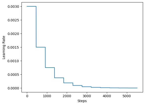
训练
对于训练,作者建议使用学习率衰减计划,即每 20 个 epoch 将初始学习率减半。在本例中,我们使用 5 个 epoch。
steps_per_epoch = total_training_examples // BATCH_SIZE
total_training_steps = steps_per_epoch * EPOCHS
print(f"Steps per epoch: {steps_per_epoch}.")
print(f"Total training steps: {total_training_steps}.")

lr_schedule = keras.optimizers.schedules.ExponentialDecay(
    initial_learning_rate=0.003,
    decay_steps=steps_per_epoch * 5,
    decay_rate=0.5,
    staircase=True,
)

steps = range(total_training_steps)
lrs = [lr_schedule(step) for step in steps]

plt.plot(lrs)
plt.xlabel("Steps")
plt.ylabel("Learning Rate")
plt.show()
Steps per epoch: 92.
Total training steps: 5520.
最后,我们实现一个用于运行实验的实用程序并启动模型训练。
def run_experiment(epochs):
    segmentation_model = get_shape_segmentation_model(num_points, num_classes)
    segmentation_model.compile(
        optimizer=keras.optimizers.Adam(learning_rate=lr_schedule),
        loss=keras.losses.CategoricalCrossentropy(),
        metrics=["accuracy"],
    )

    checkpoint_filepath = "checkpoint.weights.h5"
    checkpoint_callback = keras.callbacks.ModelCheckpoint(
        checkpoint_filepath,
        monitor="val_loss",
        save_best_only=True,
        save_weights_only=True,
    )

    history = segmentation_model.fit(
        train_dataset,
        validation_data=val_dataset,
        epochs=epochs,
        callbacks=[checkpoint_callback],
    )

    segmentation_model.load_weights(checkpoint_filepath)
    return segmentation_model, history


segmentation_model, history = run_experiment(epochs=EPOCHS)
Epoch 1/60
2/93 [37m━━━━━━━━━━━━━━━━━━━━ 7s 86ms/step - accuracy: 0.1427 - loss: 48748.8203
WARNING: All log messages before absl::InitializeLog() is called are written to STDERR
I0000 00:00:1699916678.434176 90326 device_compiler.h:187] Compiled cluster using XLA! This line is logged at most once for the lifetime of the process.
93/93 ━━━━━━━━━━━━━━━━━━━━ 53s 259ms/step - accuracy: 0.3739 - loss: 27980.7305 - val_accuracy: 0.4340 - val_loss: 10361231.0000
Epoch 2/60
93/93 ━━━━━━━━━━━━━━━━━━━━ 48s 82ms/step - accuracy: 0.6355 - loss: 339.9151 - val_accuracy: 0.3820 - val_loss: 19069320.0000
Epoch 3/60
93/93 ━━━━━━━━━━━━━━━━━━━━ 8s 82ms/step - accuracy: 0.6695 - loss: 281.5728 - val_accuracy: 0.2859 - val_loss: 15993839.0000
Epoch 4/60
93/93 ━━━━━━━━━━━━━━━━━━━━ 8s 89ms/step - accuracy: 0.6812 - loss: 253.0939 - val_accuracy: 0.2287 - val_loss: 9633191.0000
Epoch 5/60
93/93 ━━━━━━━━━━━━━━━━━━━━ 8s 89ms/step - accuracy: 0.6873 - loss: 231.1317 - val_accuracy: 0.3030 - val_loss: 6001454.0000
Epoch 6/60
93/93 ━━━━━━━━━━━━━━━━━━━━ 8s 88ms/step - accuracy: 0.6860 - loss: 216.6793 - val_accuracy: 0.0620 - val_loss: 1945100.8750
Epoch 7/60
93/93 ━━━━━━━━━━━━━━━━━━━━ 8s 82ms/step - accuracy: 0.6947 - loss: 210.2683 - val_accuracy: 0.4539 - val_loss: 7908162.5000
Epoch 8/60
93/93 ━━━━━━━━━━━━━━━━━━━━ 8s 82ms/step - accuracy: 0.7014 - loss: 203.2560 - val_accuracy: 0.4035 - val_loss: 17741164.0000
Epoch 9/60
93/93 ━━━━━━━━━━━━━━━━━━━━ 8s 82ms/step - accuracy: 0.7006 - loss: 197.3710 - val_accuracy: 0.1900 - val_loss: 34120616.0000
Epoch 10/60
93/93 ━━━━━━━━━━━━━━━━━━━━ 8s 82ms/step - accuracy: 0.7047 - loss: 192.0777 - val_accuracy: 0.3391 - val_loss: 33157422.0000
Epoch 11/60
93/93 ━━━━━━━━━━━━━━━━━━━━ 8s 82ms/step - accuracy: 0.7102 - loss: 188.4875 - val_accuracy: 0.3394 - val_loss: 4630613.5000
Epoch 12/60
93/93 ━━━━━━━━━━━━━━━━━━━━ 8s 89ms/step - accuracy: 0.7186 - loss: 184.9940 - val_accuracy: 0.1662 - val_loss: 487790.1250
Epoch 13/60
93/93 ━━━━━━━━━━━━━━━━━━━━ 8s 89ms/step - accuracy: 0.7175 - loss: 182.7206 - val_accuracy: 0.1602 - val_loss: 70590.3203
Epoch 14/60
93/93 ━━━━━━━━━━━━━━━━━━━━ 8s 88ms/step - accuracy: 0.7159 - loss: 180.5028 - val_accuracy: 0.1631 - val_loss: 16990.2324
Epoch 15/60
93/93 ━━━━━━━━━━━━━━━━━━━━ 8s 88ms/step - accuracy: 0.7201 - loss: 180.1674 - val_accuracy: 0.2318 - val_loss: 4992.7783
Epoch 16/60
93/93 ━━━━━━━━━━━━━━━━━━━━ 8s 88ms/step - accuracy: 0.7222 - loss: 176.5523 - val_accuracy: 0.6246 - val_loss: 647.5634
Epoch 17/60
93/93 ━━━━━━━━━━━━━━━━━━━━ 8s 88ms/step - accuracy: 0.7291 - loss: 175.6139 - val_accuracy: 0.6551 - val_loss: 324.0956
Epoch 18/60
93/93 ━━━━━━━━━━━━━━━━━━━━ 8s 88ms/step - accuracy: 0.7285 - loss: 175.0228 - val_accuracy: 0.6430 - val_loss: 257.9340
Epoch 19/60
93/93 ━━━━━━━━━━━━━━━━━━━━ 8s 88ms/step - accuracy: 0.7300 - loss: 172.7668 - val_accuracy: 0.6399 - val_loss: 253.2745
Epoch 20/60
93/93 ━━━━━━━━━━━━━━━━━━━━ 8s 89ms/step - accuracy: 0.7316 - loss: 172.9001 - val_accuracy: 0.6084 - val_loss: 232.9293
Epoch 21/60
93/93 ━━━━━━━━━━━━━━━━━━━━ 8s 89ms/step - accuracy: 0.7364 - loss: 170.8767 - val_accuracy: 0.6451 - val_loss: 191.7183
Epoch 22/60
93/93 ━━━━━━━━━━━━━━━━━━━━ 8s 88ms/step - accuracy: 0.7395 - loss: 171.4525 - val_accuracy: 0.6825 - val_loss: 180.2473
Epoch 23/60
93/93 ━━━━━━━━━━━━━━━━━━━━ 8s 82ms/step - accuracy: 0.7392 - loss: 170.1975 - val_accuracy: 0.6095 - val_loss: 180.3243
Epoch 24/60
93/93 ━━━━━━━━━━━━━━━━━━━━ 8s 88ms/step - accuracy: 0.7362 - loss: 169.2144 - val_accuracy: 0.6017 - val_loss: 178.3013
Epoch 25/60
93/93 ━━━━━━━━━━━━━━━━━━━━ 8s 82ms/step - accuracy: 0.7409 - loss: 169.2571 - val_accuracy: 0.6582 - val_loss: 178.3481
Epoch 26/60
93/93 ━━━━━━━━━━━━━━━━━━━━ 8s 89ms/step - accuracy: 0.7415 - loss: 167.7480 - val_accuracy: 0.6808 - val_loss: 177.8774
Epoch 27/60
93/93 ━━━━━━━━━━━━━━━━━━━━ 8s 89ms/step - accuracy: 0.7440 - loss: 167.7844 - val_accuracy: 0.7131 - val_loss: 176.5841
Epoch 28/60
93/93 ━━━━━━━━━━━━━━━━━━━━ 8s 88ms/step - accuracy: 0.7423 - loss: 167.5307 - val_accuracy: 0.6891 - val_loss: 176.1687
Epoch 29/60
93/93 ━━━━━━━━━━━━━━━━━━━━ 8s 88ms/step - accuracy: 0.7409 - loss: 166.4581 - val_accuracy: 0.7136 - val_loss: 174.9417
Epoch 30/60
93/93 ━━━━━━━━━━━━━━━━━━━━ 8s 88ms/step - accuracy: 0.7419 - loss: 165.9243 - val_accuracy: 0.7407 - val_loss: 173.0663
Epoch 31/60
93/93 ━━━━━━━━━━━━━━━━━━━━ 8s 88ms/step - accuracy: 0.7471 - loss: 166.9746 - val_accuracy: 0.7454 - val_loss: 172.9663
Epoch 32/60
93/93 ━━━━━━━━━━━━━━━━━━━━ 8s 82ms/step - accuracy: 0.7472 - loss: 165.9707 - val_accuracy: 0.7480 - val_loss: 173.9868
Epoch 33/60
93/93 ━━━━━━━━━━━━━━━━━━━━ 8s 82ms/step - accuracy: 0.7443 - loss: 165.9368 - val_accuracy: 0.7076 - val_loss: 174.4526
Epoch 34/60
93/93 ━━━━━━━━━━━━━━━━━━━━ 8s 82ms/step - accuracy: 0.7496 - loss: 165.5322 - val_accuracy: 0.7441 - val_loss: 174.6099
Epoch 35/60
93/93 ━━━━━━━━━━━━━━━━━━━━ 8s 82ms/step - accuracy: 0.7453 - loss: 164.2007 - val_accuracy: 0.7469 - val_loss: 174.2793
Epoch 36/60
93/93 ━━━━━━━━━━━━━━━━━━━━ 8s 82ms/step - accuracy: 0.7503 - loss: 165.3418 - val_accuracy: 0.7469 - val_loss: 174.0812
Epoch 37/60
93/93 ━━━━━━━━━━━━━━━━━━━━ 8s 82ms/step - accuracy: 0.7491 - loss: 164.4796 - val_accuracy: 0.7524 - val_loss: 173.9656
Epoch 38/60
93/93 ━━━━━━━━━━━━━━━━━━━━ 10s 82ms/step - accuracy: 0.7489 - loss: 164.4573 - val_accuracy: 0.7516 - val_loss: 175.3401
Epoch 39/60
93/93 ━━━━━━━━━━━━━━━━━━━━ 8s 82ms/step - accuracy: 0.7437 - loss: 163.4484 - val_accuracy: 0.7532 - val_loss: 173.8172
Epoch 40/60
93/93 ━━━━━━━━━━━━━━━━━━━━ 8s 82ms/step - accuracy: 0.7507 - loss: 163.6720 - val_accuracy: 0.7537 - val_loss: 173.9127
Epoch 41/60
93/93 ━━━━━━━━━━━━━━━━━━━━ 8s 82ms/step - accuracy: 0.7506 - loss: 164.0555 - val_accuracy: 0.7556 - val_loss: 173.0979
Epoch 42/60
93/93 ━━━━━━━━━━━━━━━━━━━━ 8s 89ms/step - accuracy: 0.7517 - loss: 164.1554 - val_accuracy: 0.7562 - val_loss: 172.8895
Epoch 43/60
93/93 ━━━━━━━━━━━━━━━━━━━━ 10s 82ms/step - accuracy: 0.7527 - loss: 164.6351 - val_accuracy: 0.7567 - val_loss: 173.0476
Epoch 44/60
93/93 ━━━━━━━━━━━━━━━━━━━━ 8s 88ms/step - accuracy: 0.7505 - loss: 164.1568 - val_accuracy: 0.7571 - val_loss: 172.2751
Epoch 45/60
93/93 ━━━━━━━━━━━━━━━━━━━━ 8s 88ms/step - accuracy: 0.7500 - loss: 163.8129 - val_accuracy: 0.7579 - val_loss: 171.8897
Epoch 46/60
93/93 ━━━━━━━━━━━━━━━━━━━━ 8s 82ms/step - accuracy: 0.7534 - loss: 163.6473 - val_accuracy: 0.7577 - val_loss: 172.5457
Epoch 47/60
93/93 ━━━━━━━━━━━━━━━━━━━━ 8s 82ms/step - accuracy: 0.7510 - loss: 163.7318 - val_accuracy: 0.7580 - val_loss: 172.2256
Epoch 48/60
93/93 ━━━━━━━━━━━━━━━━━━━━ 8s 82ms/step - accuracy: 0.7517 - loss: 163.3274 - val_accuracy: 0.7575 - val_loss: 172.3276
Epoch 49/60
93/93 ━━━━━━━━━━━━━━━━━━━━ 8s 89ms/step - accuracy: 0.7511 - loss: 163.5069 - val_accuracy: 0.7581 - val_loss: 171.2155
Epoch 50/60
93/93 ━━━━━━━━━━━━━━━━━━━━ 8s 89ms/step - accuracy: 0.7507 - loss: 163.7366 - val_accuracy: 0.7578 - val_loss: 171.1100
Epoch 51/60
93/93 ━━━━━━━━━━━━━━━━━━━━ 8s 82ms/step - accuracy: 0.7519 - loss: 163.1190 - val_accuracy: 0.7580 - val_loss: 171.7971
Epoch 52/60
93/93 ━━━━━━━━━━━━━━━━━━━━ 8s 81ms/step - accuracy: 0.7510 - loss: 162.7351 - val_accuracy: 0.7579 - val_loss: 171.9780
Epoch 53/60
93/93 ━━━━━━━━━━━━━━━━━━━━ 8s 82ms/step - accuracy: 0.7510 - loss: 162.9639 - val_accuracy: 0.7577 - val_loss: 171.6770
Epoch 54/60
93/93 ━━━━━━━━━━━━━━━━━━━━ 8s 88ms/step - accuracy: 0.7530 - loss: 162.7419 - val_accuracy: 0.7578 - val_loss: 170.5556
Epoch 55/60
93/93 ━━━━━━━━━━━━━━━━━━━━ 8s 82ms/step - accuracy: 0.7515 - loss: 163.2893 - val_accuracy: 0.7582 - val_loss: 171.9172
Epoch 56/60
93/93 ━━━━━━━━━━━━━━━━━━━━ 8s 82ms/step - accuracy: 0.7505 - loss: 164.2843 - val_accuracy: 0.7584 - val_loss: 171.9182
Epoch 57/60
93/93 ━━━━━━━━━━━━━━━━━━━━ 8s 82ms/step - accuracy: 0.7498 - loss: 162.6679 - val_accuracy: 0.7587 - val_loss: 173.7610
Epoch 58/60
93/93 ━━━━━━━━━━━━━━━━━━━━ 8s 82ms/step - accuracy: 0.7523 - loss: 163.3332 - val_accuracy: 0.7585 - val_loss: 172.5207
Epoch 59/60
93/93 ━━━━━━━━━━━━━━━━━━━━ 8s 82ms/step - accuracy: 0.7529 - loss: 162.4575 - val_accuracy: 0.7586 - val_loss: 171.6861
Epoch 60/60
93/93 ━━━━━━━━━━━━━━━━━━━━ 8s 82ms/step - accuracy: 0.7498 - loss: 162.9523 - val_accuracy: 0.7586 - val_loss: 172.3012
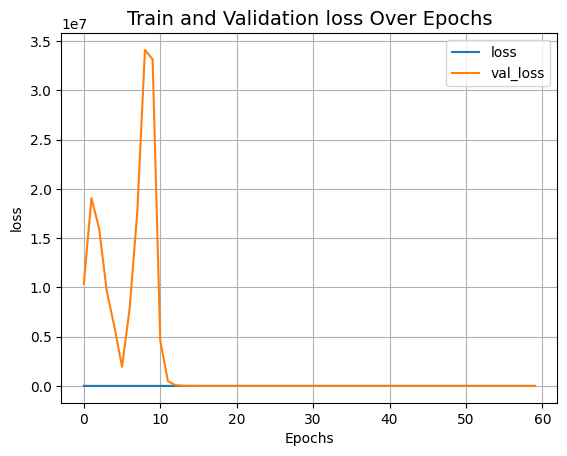
可视化训练过程
def plot_result(item):
plt.plot(history.history[item], label=item)
plt.plot(history.history["val_" + item], label="val_" + item)
plt.xlabel("Epochs")
plt.ylabel(item)
plt.title("Train and Validation {} Over Epochs".format(item), fontsize=14)
plt.legend()
plt.grid()
plt.show()
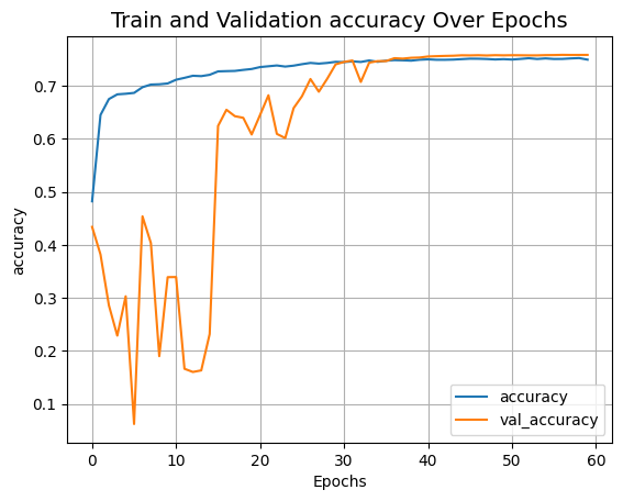
plot_result("loss")
plot_result("accuracy")
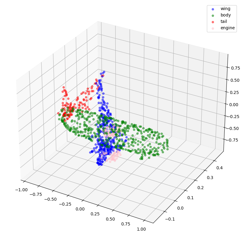
推理
validation_batch = next(iter(val_dataset))
val_predictions = segmentation_model.predict(validation_batch[0])
print(f"Validation prediction shape: {val_predictions.shape}")
def visualize_single_point_cloud(point_clouds, label_clouds, idx):
label_map = LABELS + ["none"]
point_cloud = point_clouds[idx]
label_cloud = label_clouds[idx]
visualize_data(point_cloud, [label_map[np.argmax(label)] for label in label_cloud])
idx = np.random.choice(len(validation_batch[0]))
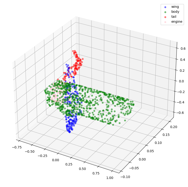
print(f"Index selected: {idx}")
# Plotting with ground-truth.
visualize_single_point_cloud(validation_batch[0], validation_batch[1], idx)
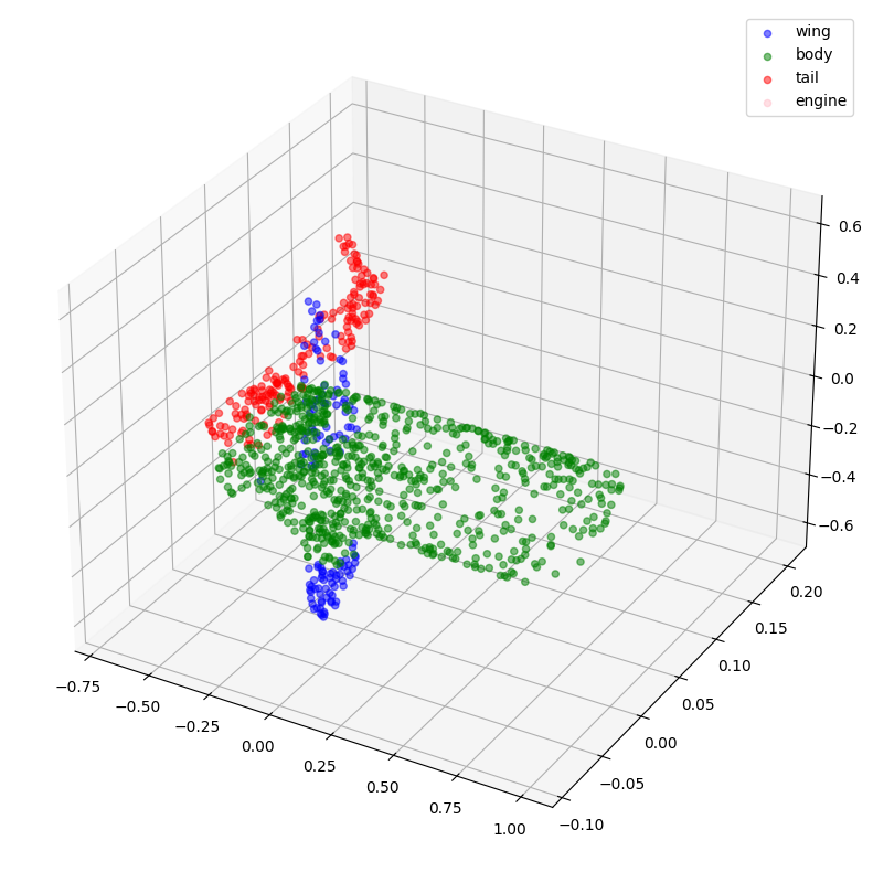
# Plotting with predicted labels.
visualize_single_point_cloud(validation_batch[0], val_predictions, idx)
 1/1 ━━━━━━━━━━━━━━━━━━━━ 1s 1s/step
Validation prediction shape: (32, 1024, 5)
Index selected: 26
结语
如果您对该主题感兴趣,可能会发现 此仓库 有用。