使用 TensorFlow Similarity 进行图像相似性搜索的度量学习
作者: Owen Vallis
创建日期 2021/09/30
最后修改日期 2022/02/29
描述: 使用 CIFAR-10 图像进行相似性度量学习的示例。

概述
本示例基于 “图像相似性搜索的度量学习”示例。我们旨在数据集相同,但使用 TensorFlow Similarity 来实现模型。
度量学习旨在训练模型,将输入嵌入到高维空间中,使得“相似”的输入彼此靠近,“不相似”的输入彼此远离。一旦训练完成,这些模型就可以为下游系统生成嵌入,这些系统可能需要这种相似性,例如作为搜索的排名信号,或者作为另一种监督问题的预训练嵌入模型。
有关度量学习的更详细概述,请参阅
设置
本教程将使用 TensorFlow Similarity 库来学习和评估相似性嵌入。TensorFlow Similarity 提供了以下组件:
- 使对比模型的训练变得简单快捷。
- 使确保批次包含示例对更容易。
- 能够评估嵌入的质量。
可以通过 pip 轻松安装 TensorFlow Similarity,如下所示
pip -q install tensorflow_similarity
import random

from matplotlib import pyplot as plt
from mpl_toolkits import axes_grid1
import numpy as np

import tensorflow as tf
from tensorflow import keras

import tensorflow_similarity as tfsim


tfsim.utils.tf_cap_memory()

print("TensorFlow:", tf.__version__)
print("TensorFlow Similarity:", tfsim.__version__)
TensorFlow: 2.7.0
TensorFlow Similarity: 0.15.5
数据集采样器
本教程将使用 CIFAR-10 数据集。
为了使相似性模型能够高效学习,每个批次必须包含每类至少 2 个示例。
为了方便实现这一点,tf_similarity 提供了 Sampler 对象,使您能够设置类别数量和每个批次中每类的最小示例数量。
训练集和验证集将使用 TFDatasetMultiShotMemorySampler 对象创建。该对象创建一个采样器,该采样器从 TensorFlow Datasets 加载数据集,并生成包含目标类别数量和每类目标示例数量的批次。此外,我们可以将采样器限制为仅生成 class_list 中定义的类别子集,从而使我们能够在类别子集上进行训练,然后测试嵌入如何泛化到未见过类别。这在处理少样本学习问题时很有用。
以下单元格创建一个 train_ds 样本,该样本
- 从 TFDS 加载 CIFAR-10 数据集,然后选取
examples_per_class_per_batch。 - 确保采样器将类别限制为
class_list中定义的类别。 - 确保每个批次包含 10 个不同的类别,每个类别 8 个示例。
我们以相同的方式创建验证数据集,但我们将每类的总示例数限制为 100,每类的每个批次示例设置为默认值 2。
# This determines the number of classes used during training.
# Here we are using all the classes.
num_known_classes = 10
class_list = random.sample(population=range(10), k=num_known_classes)

classes_per_batch = 10
# Passing multiple examples per class per batch ensures that each example has
# multiple positive pairs. This can be useful when performing triplet mining or
# when using losses like `MultiSimilarityLoss` or `CircleLoss` as these can
# take a weighted mix of all the positive pairs. In general, more examples per
# class will lead to more information for the positive pairs, while more classes
# per batch will provide more varied information in the negative pairs. However,
# the losses compute the pairwise distance between the examples in a batch so
# the upper limit of the batch size is restricted by the memory.
examples_per_class_per_batch = 8

print(
    "Batch size is: "
    f"{min(classes_per_batch, num_known_classes) * examples_per_class_per_batch}"
)

print(" Create Training Data ".center(34, "#"))
train_ds = tfsim.samplers.TFDatasetMultiShotMemorySampler(
    "cifar10",
    classes_per_batch=min(classes_per_batch, num_known_classes),
    splits="train",
    steps_per_epoch=4000,
    examples_per_class_per_batch=examples_per_class_per_batch,
    class_list=class_list,
)

print("\n" + " Create Validation Data ".center(34, "#"))
val_ds = tfsim.samplers.TFDatasetMultiShotMemorySampler(
    "cifar10",
    classes_per_batch=classes_per_batch,
    splits="test",
    total_examples_per_class=100,
)
Batch size is: 80
###### Create Training Data ######

converting train:   0%|          | 0/50000 [00:00<?, ?it/s]
The initial batch size is 80 (10 classes * 8 examples per class) with 0 augmenters

filtering examples:   0%|          | 0/50000 [00:00<?, ?it/s]

selecting classes:   0%|          | 0/10 [00:00<?, ?it/s]

gather examples:   0%|          | 0/50000 [00:00<?, ?it/s]

indexing classes:   0%|          | 0/50000 [00:00<?, ?it/s]
##### Create Validation Data #####

converting test:   0%|          | 0/10000 [00:00<?, ?it/s]
The initial batch size is 20 (10 classes * 2 examples per class) with 0 augmenters

filtering examples:   0%|          | 0/10000 [00:00<?, ?it/s]

selecting classes:   0%|          | 0/10 [00:00<?, ?it/s]

gather examples:   0%|          | 0/1000 [00:00<?, ?it/s]

indexing classes:   0%|          | 0/1000 [00:00<?, ?it/s]
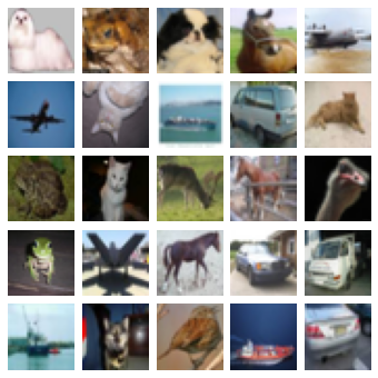
可视化数据集
采样器将对数据集进行混洗,因此我们可以通过绘制前 25 张图像来了解数据集。
采样器提供了 get_slice(begin, size) 方法,该方法允许我们轻松选择一个样本块。
或者,我们可以使用 generate_batch() 方法来生成批次。这可以让我们检查批次是否包含预期的类别数量和每类示例数量。
num_cols = num_rows = 5
# Get the first 25 examples.
x_slice, y_slice = train_ds.get_slice(begin=0, size=num_cols * num_rows)

fig = plt.figure(figsize=(6.0, 6.0))
grid = axes_grid1.ImageGrid(fig, 111, nrows_ncols=(num_cols, num_rows), axes_pad=0.1)

for ax, im, label in zip(grid, x_slice, y_slice):
    ax.imshow(im)
    ax.axis("off")
嵌入模型
接下来,我们使用 Keras Functional API 定义一个 SimilarityModel。该模型是一个标准的卷积网络,额外添加了一个 MetricEmbedding 层,该层应用 L2 归一化。当使用 Cosine 距离时,度量嵌入层很有用,因为我们只关心向量之间的角度。
此外,SimilarityModel 还提供了许多有助于
- 索引嵌入的示例
- 执行示例查找
- 评估分类
- 评估嵌入空间的质量
有关更多详细信息,请参阅 TensorFlow Similarity 文档。
embedding_size = 256

inputs = keras.layers.Input((32, 32, 3))
x = keras.layers.Rescaling(scale=1.0 / 255)(inputs)
x = keras.layers.Conv2D(64, 3, activation="relu")(x)
x = keras.layers.BatchNormalization()(x)
x = keras.layers.Conv2D(128, 3, activation="relu")(x)
x = keras.layers.BatchNormalization()(x)
x = keras.layers.MaxPool2D((4, 4))(x)
x = keras.layers.Conv2D(256, 3, activation="relu")(x)
x = keras.layers.BatchNormalization()(x)
x = keras.layers.Conv2D(256, 3, activation="relu")(x)
x = keras.layers.GlobalMaxPool2D()(x)
outputs = tfsim.layers.MetricEmbedding(embedding_size)(x)

# building model
model = tfsim.models.SimilarityModel(inputs, outputs)
model.summary()
Model: "similarity_model"
_________________________________________________________________
 Layer (type)                Output Shape              Param #
=================================================================
 input_1 (InputLayer)        [(None, 32, 32, 3)]       0

 rescaling (Rescaling)       (None, 32, 32, 3)         0

 conv2d (Conv2D)             (None, 30, 30, 64)        1792

 batch_normalization (BatchN  (None, 30, 30, 64)       256
 ormalization)

 conv2d_1 (Conv2D)           (None, 28, 28, 128)       73856

 batch_normalization_1 (Batc  (None, 28, 28, 128)      512
 hNormalization)

 max_pooling2d (MaxPooling2D  (None, 7, 7, 128)        0
 )

 conv2d_2 (Conv2D)           (None, 5, 5, 256)         295168

 batch_normalization_2 (Batc  (None, 5, 5, 256)        1024
 hNormalization)

 conv2d_3 (Conv2D)           (None, 3, 3, 256)         590080

 global_max_pooling2d (Globa  (None, 256)              0
 lMaxPooling2D)

 metric_embedding (MetricEmb  (None, 256)              65792
 edding)

=================================================================
Total params: 1,028,480
Trainable params: 1,027,584
Non-trainable params: 896
_________________________________________________________________
相似性损失
相似性损失需要每类至少包含 2 个示例的批次,从中计算出成对正负距离的损失。这里我们使用 MultiSimilarityLoss() (论文),它是 TensorFlow Similarity 中的几种损失之一。此损失尝试使用批次中的所有信息对,同时考虑自相似性、正相似性和负相似性。
epochs = 3
learning_rate = 0.002
val_steps = 50

# init similarity loss
loss = tfsim.losses.MultiSimilarityLoss()

# compiling and training
model.compile(
    optimizer=keras.optimizers.Adam(learning_rate), loss=loss, steps_per_execution=10,
)
history = model.fit(
    train_ds, epochs=epochs, validation_data=val_ds, validation_steps=val_steps
)
Distance metric automatically set to cosine use the distance arg to override.
Epoch 1/3

4000/4000 [==============================] - ETA: 0s - loss: 2.2179Warmup complete
4000/4000 [==============================] - 38s 9ms/step - loss: 2.2179 - val_loss: 0.8894
Warmup complete
Epoch 2/3
4000/4000 [==============================] - 34s 9ms/step - loss: 1.9047 - val_loss: 0.8767
Epoch 3/3
4000/4000 [==============================] - 35s 9ms/step - loss: 1.6336 - val_loss: 0.8469
索引
在训练完模型后,我们可以创建一个示例索引。这里我们将前 200 个验证示例进行批次索引,方法是将 x 和 y 传递给索引,同时将图像存储在 data 参数中。x_index 值被嵌入然后添加到索引中以便搜索。y_index 和 data 参数是可选的,但允许用户将元数据与嵌入的示例关联起来。
x_index, y_index = val_ds.get_slice(begin=0, size=200)
model.reset_index()
model.index(x_index, y_index, data=x_index)
[Indexing 200 points]
|-Computing embeddings
|-Storing data points in key value store
|-Adding embeddings to index.
|-Building index.
0%   10   20   30   40   50   60   70   80   90   100%
|----|----|----|----|----|----|----|----|----|----|
***************************************************
校准
构建索引后,我们可以使用匹配策略和校准指标来校准距离阈值。
这里我们使用 K=1 作为分类器来搜索最优 F1 分数。所有距离等于或小于校准阈值的匹配将被标记为查询示例与匹配结果关联的标签之间的正匹配,而所有大于阈值的匹配将被标记为负匹配。
此外,我们还传递了额外的指标来计算。输出中的所有值都在校准阈值下计算。
最后,model.calibrate() 返回一个 CalibrationResults 对象,其中包含
"cutpoints":一个 Python 字典,将切点名称映射到一个字典,该字典包含与特定距离阈值关联的ClassificationMetric值,例如"optimal" : {"acc": 0.90, "f1": 0.92}。"thresholds":一个 Python 字典,将ClassificationMetric名称映射到一个列表,该列表包含在每个距离阈值下计算的指标值,例如{"f1": [0.99, 0.80], "distance": [0.0, 1.0]}。
x_train, y_train = train_ds.get_slice(begin=0, size=1000)
calibration = model.calibrate(
    x_train,
    y_train,
    calibration_metric="f1",
    matcher="match_nearest",
    extra_metrics=["precision", "recall", "binary_accuracy"],
    verbose=1,
)
Performing NN search
Building NN list:   0%|          | 0/1000 [00:00<?, ?it/s]

Evaluating:   0%|          | 0/4 [00:00<?, ?it/s]

computing thresholds:   0%|          | 0/989 [00:00<?, ?it/s]
 name       value    distance    precision    recall    binary_accuracy        f1
-------  -------  ----------  -----------  --------  -----------------  --------
optimal     0.93    0.048435        0.869         1              0.869  0.929909
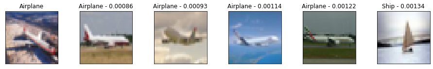
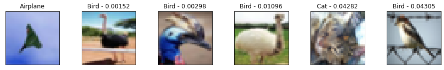
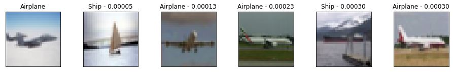
可视化
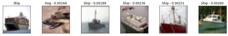
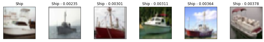
仅从指标中可能很难对模型的质量有一个直观的认识。一种互补的方法是手动检查一组查询结果,以了解匹配质量。
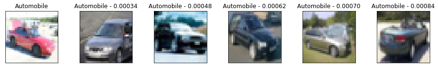
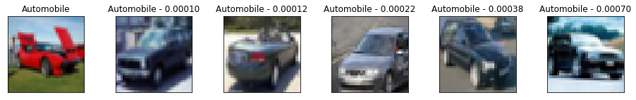
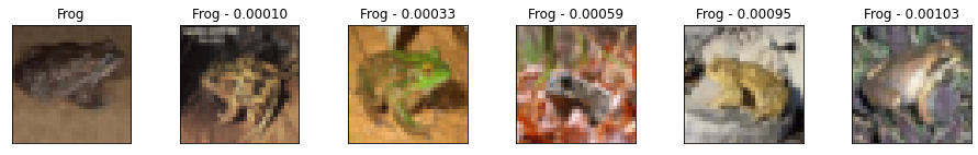
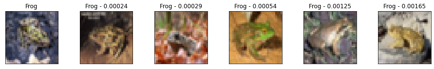
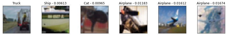
这里我们选取 10 个验证示例,并绘制它们与它们的 5 个最近邻以及到查询示例的距离。从结果可以看出,虽然它们不完美,但仍然代表有意义的相似图像,并且模型能够找到相似的图像,而不管其姿势或图像光照如何。
我们还可以看到模型对某些图像非常自信,导致查询和邻居之间的距离非常小。相反,随着距离的增加,我们在类别标签中看到更多的错误。这也是为什么校准对于匹配应用程序至关重要的一些原因。
num_neighbors = 5
labels = [
    "Airplane",
    "Automobile",
    "Bird",
    "Cat",
    "Deer",
    "Dog",
    "Frog",
    "Horse",
    "Ship",
    "Truck",
    "Unknown",
]
class_mapping = {c_id: c_lbl for c_id, c_lbl in zip(range(11), labels)}

x_display, y_display = val_ds.get_slice(begin=200, size=10)
# lookup nearest neighbors in the index
nns = model.lookup(x_display, k=num_neighbors)

# display
for idx in np.argsort(y_display):
    tfsim.visualization.viz_neigbors_imgs(
        x_display[idx],
        y_display[idx],
        nns[idx],
        class_mapping=class_mapping,
        fig_size=(16, 2),
    )
Performing NN search
Building NN list: 0%| | 0/10 [00:00<?, ?it/s]
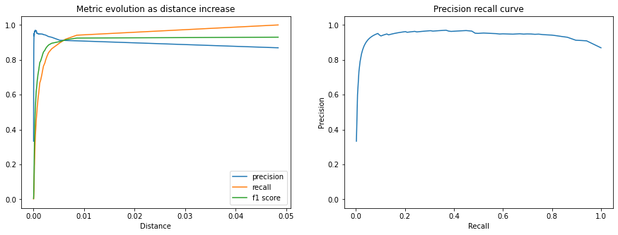
指标
我们还可以绘制 CalibrationResults 中包含的额外指标,以了解随着距离阈值的增加,匹配性能如何。
以下图表显示了精度、召回率和 F1 分数。我们可以看到,随着距离的增加,匹配精度会下降,但我们接受为正匹配的查询百分比(召回率)在校准距离阈值之前增长更快。
fig, (ax1, ax2) = plt.subplots(1, 2, figsize=(15, 5))
x = calibration.thresholds["distance"]

ax1.plot(x, calibration.thresholds["precision"], label="precision")
ax1.plot(x, calibration.thresholds["recall"], label="recall")
ax1.plot(x, calibration.thresholds["f1"], label="f1 score")
ax1.legend()
ax1.set_title("Metric evolution as distance increase")
ax1.set_xlabel("Distance")
ax1.set_ylim((-0.05, 1.05))

ax2.plot(calibration.thresholds["recall"], calibration.thresholds["precision"])
ax2.set_title("Precision recall curve")
ax2.set_xlabel("Recall")
ax2.set_ylabel("Precision")
ax2.set_ylim((-0.05, 1.05))
plt.show()
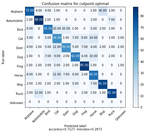
我们还可以为每个类别选取 100 个示例,并为每个示例及其最近的匹配项绘制混淆矩阵。我们还添加了一个“额外”的第 10 个类别来表示校准距离阈值以上的匹配项。
我们可以看到,大多数错误是动物类别之间的,并且飞机和鸟类之间存在有趣的混淆。此外,我们看到每个类别中只有少数 100 个示例返回了校准距离阈值之外的匹配项。
cutpoint = "optimal"

# This yields 100 examples for each class.
# We defined this when we created the val_ds sampler.
x_confusion, y_confusion = val_ds.get_slice(0, -1)

matches = model.match(x_confusion, cutpoint=cutpoint, no_match_label=10)
cm = tfsim.visualization.confusion_matrix(
    matches,
    y_confusion,
    labels=labels,
    title="Confusion matrix for cutpoint:%s" % cutpoint,
    normalize=False,
)
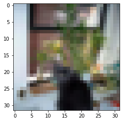
无匹配
我们可以绘制校准阈值之外的示例,以查看哪些图像未匹配任何索引的示例。
这可能有助于了解可能需要索引哪些其他示例,或者发现类别内的异常示例。
idx_no_match = np.where(np.array(matches) == 10)
no_match_queries = x_confusion[idx_no_match]
if len(no_match_queries):
    plt.imshow(no_match_queries[0])
else:
    print("All queries have a match below the distance threshold.")
可视化聚类
快速了解模型表现质量并理解其不足之处的最佳方法之一是将嵌入投影到 2D 空间。
这使我们能够检查图像簇并了解哪些类别是纠缠的。
# Each class in val_ds was restricted to 100 examples.
num_examples_to_clusters = 1000
thumb_size = 96
plot_size = 800
vx, vy = val_ds.get_slice(0, num_examples_to_clusters)

# Uncomment to run the interactive projector.
# tfsim.visualization.projector(
#     model.predict(vx),
#     labels=vy,
#     images=vx,
#     class_mapping=class_mapping,
#     image_size=thumb_size,
#     plot_size=plot_size,
# )