图像相似性搜索的度量学习
作者: Mat Kelcey
创建日期 2020/06/05
最后修改日期 2020/06/09
描述: 在CIFAR-10图像上使用相似性度量学习的示例。

概述
度量学习旨在训练模型,将输入嵌入到高维空间中,使得由训练方案定义的“相似”输入彼此靠近。一旦这些模型训练完毕,就可以为需要这种相似性的下游系统生成嵌入;例如,作为搜索的排名信号,或者作为另一种有监督问题的预训练嵌入模型的形式。
有关度量学习的更详细概述,请参阅
设置
将Keras后端设置为tensorflow。
import os

os.environ["KERAS_BACKEND"] = "tensorflow"

import random
import matplotlib.pyplot as plt
import numpy as np
import tensorflow as tf
from collections import defaultdict
from PIL import Image
from sklearn.metrics import ConfusionMatrixDisplay
import keras
from keras import layers
数据集
在这个示例中,我们将使用CIFAR-10数据集。
from keras.datasets import cifar10


(x_train, y_train), (x_test, y_test) = cifar10.load_data()

x_train = x_train.astype("float32") / 255.0
y_train = np.squeeze(y_train)
x_test = x_test.astype("float32") / 255.0
y_test = np.squeeze(y_test)
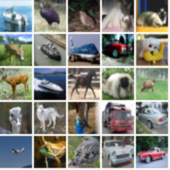
为了了解数据集,我们可以可视化25个随机示例的网格。
height_width = 32


def show_collage(examples):
    box_size = height_width + 2
    num_rows, num_cols = examples.shape[:2]

    collage = Image.new(
        mode="RGB",
        size=(num_cols * box_size, num_rows * box_size),
        color=(250, 250, 250),
    )
    for row_idx in range(num_rows):
        for col_idx in range(num_cols):
            array = (np.array(examples[row_idx, col_idx]) * 255).astype(np.uint8)
            collage.paste(
                Image.fromarray(array), (col_idx * box_size, row_idx * box_size)
            )

    # Double size for visualisation.
    collage = collage.resize((2 * num_cols * box_size, 2 * num_rows * box_size))
    return collage


# Show a collage of 5x5 random images.
sample_idxs = np.random.randint(0, 50000, size=(5, 5))
examples = x_train[sample_idxs]
show_collage(examples)
度量学习提供的训练数据不是显式的(X, y)对,而是使用我们希望表达相似性的多个实例。在我们的示例中,我们将使用相同类别的实例来表示相似性;单个训练实例不是一张图像,而是同一类别的两张图像。在引用这对图像时,我们将使用常见的度量学习术语:anchor(随机选择的图像)和positive(同一类别的另一张随机选择的图像)。
为了实现这一点,我们需要构建一种将类别映射到该类别实例的查找机制。在生成训练数据时,我们将从该查找中采样。
class_idx_to_train_idxs = defaultdict(list)
for y_train_idx, y in enumerate(y_train):
    class_idx_to_train_idxs[y].append(y_train_idx)

class_idx_to_test_idxs = defaultdict(list)
for y_test_idx, y in enumerate(y_test):
    class_idx_to_test_idxs[y].append(y_test_idx)
在这个示例中,我们使用的是最简单的训练方法;一个批次将由跨类别的(anchor, positive)对组成。学习的目标是让anchor和positive对彼此靠近,并远离批次中的其他实例。在这种情况下,批次大小将由类别数量决定;对于CIFAR-10,这是10。
num_classes = 10


class AnchorPositivePairs(keras.utils.Sequence):
    def __init__(self, num_batches):
        super().__init__()
        self.num_batches = num_batches

    def __len__(self):
        return self.num_batches

    def __getitem__(self, _idx):
        x = np.empty((2, num_classes, height_width, height_width, 3), dtype=np.float32)
        for class_idx in range(num_classes):
            examples_for_class = class_idx_to_train_idxs[class_idx]
            anchor_idx = random.choice(examples_for_class)
            positive_idx = random.choice(examples_for_class)
            while positive_idx == anchor_idx:
                positive_idx = random.choice(examples_for_class)
            x[0, class_idx] = x_train[anchor_idx]
            x[1, class_idx] = x_train[positive_idx]
        return x
我们可以通过另一个拼贴画来可视化一个批次。顶行显示从10个类别中随机选择的anchors,底行显示相应的10个positives。
examples = next(iter(AnchorPositivePairs(num_batches=1)))

show_collage(examples)

嵌入模型
我们定义了一个自定义模型,其train_step首先嵌入anchors和positives,然后使用它们成对的点积作为softmax的logits。
class EmbeddingModel(keras.Model):
    def train_step(self, data):
        # Note: Workaround for open issue, to be removed.
        if isinstance(data, tuple):
            data = data[0]
        anchors, positives = data[0], data[1]

        with tf.GradientTape() as tape:
            # Run both anchors and positives through model.
            anchor_embeddings = self(anchors, training=True)
            positive_embeddings = self(positives, training=True)

            # Calculate cosine similarity between anchors and positives. As they have
            # been normalised this is just the pair wise dot products.
            similarities = keras.ops.einsum(
                "ae,pe->ap", anchor_embeddings, positive_embeddings
            )

            # Since we intend to use these as logits we scale them by a temperature.
            # This value would normally be chosen as a hyper parameter.
            temperature = 0.2
            similarities /= temperature

            # We use these similarities as logits for a softmax. The labels for
            # this call are just the sequence [0, 1, 2, ..., num_classes] since we
            # want the main diagonal values, which correspond to the anchor/positive
            # pairs, to be high. This loss will move embeddings for the
            # anchor/positive pairs together and move all other pairs apart.
            sparse_labels = keras.ops.arange(num_classes)
            loss = self.compute_loss(y=sparse_labels, y_pred=similarities)

        # Calculate gradients and apply via optimizer.
        gradients = tape.gradient(loss, self.trainable_variables)
        self.optimizer.apply_gradients(zip(gradients, self.trainable_variables))

        # Update and return metrics (specifically the one for the loss value).
        for metric in self.metrics:
            # Calling `self.compile` will by default add a [`keras.metrics.Mean`](/api/metrics/metrics_wrappers#mean-class) loss
            if metric.name == "loss":
                metric.update_state(loss)
            else:
                metric.update_state(sparse_labels, similarities)

        return {m.name: m.result() for m in self.metrics}
接下来,我们描述将图像映射到嵌入的架构。该模型仅由一系列2D卷积、全局池化和一个最终线性投影到嵌入空间组成。正如在度量学习中常见的那样,我们对嵌入进行归一化,以便使用简单的点积来衡量相似性。为了简化起见,该模型故意做得较小。
inputs = layers.Input(shape=(height_width, height_width, 3))
x = layers.Conv2D(filters=32, kernel_size=3, strides=2, activation="relu")(inputs)
x = layers.Conv2D(filters=64, kernel_size=3, strides=2, activation="relu")(x)
x = layers.Conv2D(filters=128, kernel_size=3, strides=2, activation="relu")(x)
x = layers.GlobalAveragePooling2D()(x)
embeddings = layers.Dense(units=8, activation=None)(x)
embeddings = layers.UnitNormalization()(embeddings)

model = EmbeddingModel(inputs, embeddings)
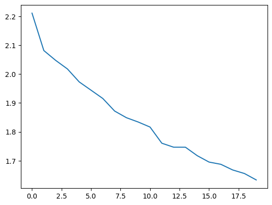
最后,我们运行训练。在Google Colab GPU实例上,这大约需要一分钟。
model.compile(
    optimizer=keras.optimizers.Adam(learning_rate=1e-3),
    loss=keras.losses.SparseCategoricalCrossentropy(from_logits=True),
)

history = model.fit(AnchorPositivePairs(num_batches=1000), epochs=20)

plt.plot(history.history["loss"])
plt.show()
Epoch 1/20
77/1000 ━[37m━━━━━━━━━━━━━━━━━━━ 1s 2ms/step - loss: 2.2962
WARNING: All log messages before absl::InitializeLog() is called are written to STDERR
I0000 00:00:1700589927.295343 3724442 device_compiler.h:187] Compiled cluster using XLA! This line is logged at most once for the lifetime of the process.
1000/1000 ━━━━━━━━━━━━━━━━━━━━ 6s 2ms/step - loss: 2.2504
Epoch 2/20
1000/1000 ━━━━━━━━━━━━━━━━━━━━ 2s 2ms/step - loss: 2.1068
Epoch 3/20
1000/1000 ━━━━━━━━━━━━━━━━━━━━ 2s 2ms/step - loss: 2.0646
Epoch 4/20
1000/1000 ━━━━━━━━━━━━━━━━━━━━ 2s 2ms/step - loss: 2.0210
Epoch 5/20
1000/1000 ━━━━━━━━━━━━━━━━━━━━ 2s 2ms/step - loss: 1.9857
Epoch 6/20
1000/1000 ━━━━━━━━━━━━━━━━━━━━ 2s 2ms/step - loss: 1.9543
Epoch 7/20
1000/1000 ━━━━━━━━━━━━━━━━━━━━ 2s 2ms/step - loss: 1.9175
Epoch 8/20
1000/1000 ━━━━━━━━━━━━━━━━━━━━ 2s 2ms/step - loss: 1.8740
Epoch 9/20
1000/1000 ━━━━━━━━━━━━━━━━━━━━ 2s 2ms/step - loss: 1.8474
Epoch 10/20
1000/1000 ━━━━━━━━━━━━━━━━━━━━ 2s 2ms/step - loss: 1.8380
Epoch 11/20
1000/1000 ━━━━━━━━━━━━━━━━━━━━ 2s 2ms/step - loss: 1.8146
Epoch 12/20
1000/1000 ━━━━━━━━━━━━━━━━━━━━ 2s 2ms/step - loss: 1.7658
Epoch 13/20
1000/1000 ━━━━━━━━━━━━━━━━━━━━ 2s 2ms/step - loss: 1.7512
Epoch 14/20
1000/1000 ━━━━━━━━━━━━━━━━━━━━ 2s 2ms/step - loss: 1.7671
Epoch 15/20
1000/1000 ━━━━━━━━━━━━━━━━━━━━ 2s 2ms/step - loss: 1.7245
Epoch 16/20
1000/1000 ━━━━━━━━━━━━━━━━━━━━ 2s 2ms/step - loss: 1.7001
Epoch 17/20
1000/1000 ━━━━━━━━━━━━━━━━━━━━ 2s 2ms/step - loss: 1.7099
Epoch 18/20
1000/1000 ━━━━━━━━━━━━━━━━━━━━ 2s 2ms/step - loss: 1.6775
Epoch 19/20
1000/1000 ━━━━━━━━━━━━━━━━━━━━ 2s 2ms/step - loss: 1.6547
Epoch 20/20
1000/1000 ━━━━━━━━━━━━━━━━━━━━ 2s 2ms/step - loss: 1.6356
测试
通过将模型应用于测试集并考虑嵌入空间中的近邻,我们可以检查模型的质量。
首先,我们嵌入测试集并计算所有近邻。请记住,由于嵌入是单位长度的,我们可以通过点积计算余弦相似性。
near_neighbours_per_example = 10

embeddings = model.predict(x_test)
gram_matrix = np.einsum("ae,be->ab", embeddings, embeddings)
near_neighbours = np.argsort(gram_matrix.T)[:, -(near_neighbours_per_example + 1) :]
313/313 ━━━━━━━━━━━━━━━━━━━━ 1s 3ms/step
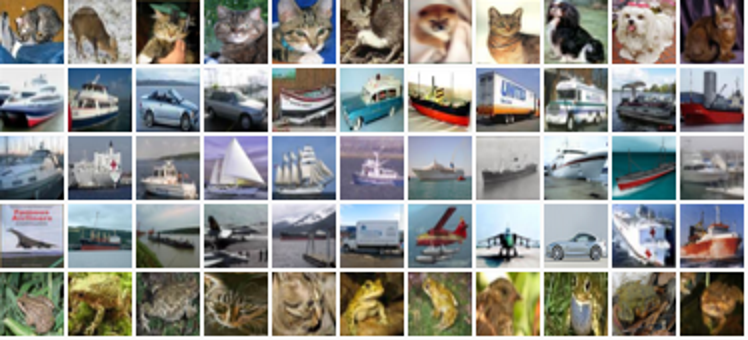
为了直观地检查这些嵌入,我们可以为5个随机示例构建近邻的拼贴画。下图的第一列是随机选择的图像,接下来的10列按相似性顺序显示最近邻。
num_collage_examples = 5

examples = np.empty(
    (
        num_collage_examples,
        near_neighbours_per_example + 1,
        height_width,
        height_width,
        3,
    ),
    dtype=np.float32,
)
for row_idx in range(num_collage_examples):
    examples[row_idx, 0] = x_test[row_idx]
    anchor_near_neighbours = reversed(near_neighbours[row_idx][:-1])
    for col_idx, nn_idx in enumerate(anchor_near_neighbours):
        examples[row_idx, col_idx + 1] = x_test[nn_idx]

show_collage(examples)
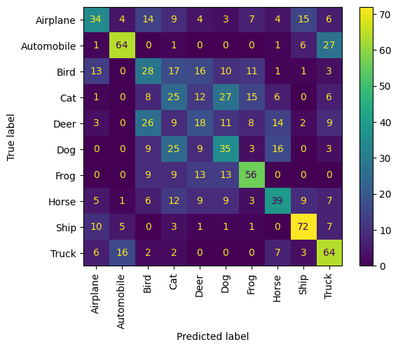
我们还可以通过考虑近邻在混淆矩阵中的正确性来获得量化的性能视图。
让我们从10个类别中每个类别采样10个示例,并将它们的近邻视为一种预测;也就是说,该示例及其近邻是否共享同一类别?
我们观察到每个动物类别通常表现良好,并且最常与其他动物类别混淆。车辆类别遵循相同的模式。
confusion_matrix = np.zeros((num_classes, num_classes))

# For each class.
for class_idx in range(num_classes):
    # Consider 10 examples.
    example_idxs = class_idx_to_test_idxs[class_idx][:10]
    for y_test_idx in example_idxs:
        # And count the classes of its near neighbours.
        for nn_idx in near_neighbours[y_test_idx][:-1]:
            nn_class_idx = y_test[nn_idx]
            confusion_matrix[class_idx, nn_class_idx] += 1

# Display a confusion matrix.
labels = [
    "Airplane",
    "Automobile",
    "Bird",
    "Cat",
    "Deer",
    "Dog",
    "Frog",
    "Horse",
    "Ship",
    "Truck",
]
disp = ConfusionMatrixDisplay(confusion_matrix=confusion_matrix, display_labels=labels)
disp.plot(include_values=True, cmap="viridis", ax=None, xticks_rotation="vertical")
plt.show()