► 代码示例 / 计算机视觉 / 使用全局上下文 Vision Transformer 进行图像分类

使用全局上下文 Vision Transformer 进行图像分类

作者：Md Awsafur Rahman
创建日期 2023/10/30
最后修改日期 2023/10/30
描述： 实现并微调用于图像分类的全局上下文 Vision Transformer。

ⓘ 本示例使用 Keras 3

设置

!pip install --upgrade keras_cv tensorflow
!pip install --upgrade keras

import keras
from keras_cv.layers import DropPath
from keras import ops
from keras import layers

import tensorflow as tf  # only for dataloader
import tensorflow_datasets as tfds  # for flower dataset

from skimage.data import chelsea
import matplotlib.pyplot as plt
import numpy as np

简介

在本 notebook 中，我们将利用多后端 Keras 3.0 实现 A Hatamizadeh 等人在 ICML 2023 上发表的 GCViT：全局上下文 Vision Transformer 论文。然后，我们将利用官方的 ImageNet 预训练权重，在 Flower 数据集上对模型进行微调，以进行图像分类任务。本 notebook 的亮点在于其与 TensorFlow、PyTorch 和 JAX 等多个后端兼容，展示了多后端 Keras 的真正潜力。

动机

注意：在本节中，我们将了解 GCViT 的背景故事，并尝试理解它为何被提出。

近年来，Transformer 在 自然语言处理 (NLP) 任务中占据主导地位，其 自注意力 机制能够捕获长距离和短距离信息。
顺应这一趋势，Vision Transformer (ViT) 提出了将图像块视为 token，并将其放入一个与原始 Transformer 编码器类似的大型架构中。
尽管 卷积神经网络 (CNN) 在计算机视觉领域长期占据主导地位，但 基于 ViT 的模型在各种计算机视觉任务中已显示出 SOTA 或具有竞争力的性能。

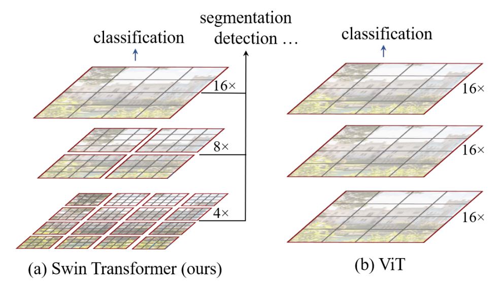
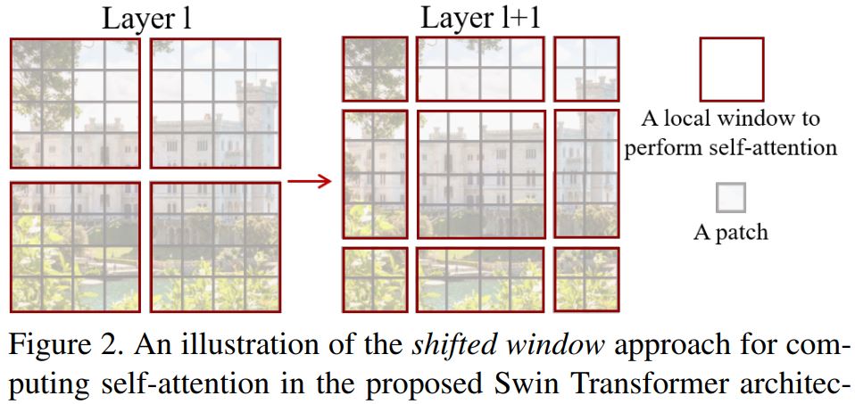
然而，自注意力的二次计算复杂度 [O(n^2)] 和缺乏多尺度信息使得 ViT 难以成为计算机视觉任务（如分割和目标检测，需要像素级别的密集预测）的通用架构。
Swin Transformer 通过提出多分辨率/分层架构来解决 ViT 的问题，在该架构中，自注意力在局部窗口内计算，并通过窗口移动等跨窗口连接来建模不同区域之间的交互。但是，局部窗口的有限感受野无法捕获长距离信息，而窗口移动等跨窗口连接方案仅覆盖每个窗口附近的一小部分邻域。此外，它还缺乏一种能够促进某种平移不变性的归纳偏置，这对于通用视觉建模，尤其是在目标检测和语义分割的密集预测任务中，仍然是可取的。

为了解决上述限制，提出了全局上下文 (GC) ViT 网络。

架构

让我们快速概览一下我们的关键组件：1. Stem/PatchEmbed：一个 stem/patchify 层在网络开始时处理图像。对于此网络，它会创建图像块/token 并将其转换为嵌入。2. Level：这是提取特征的重复构建块，使用不同的块。3. Global Token Gen./FeatureExtraction：它使用深度卷积 CNN、SqueezeAndExcitation (SE)、CNN 和MaxPooling 来生成全局 token/图像块。因此，它基本上是一个特征提取器。4. Block：这是对特征应用注意力并将它们投影到特定维度的重复模块。1. Local-MSA：局部多头自注意力。2. Global-MSA：全局多头自注意力。3. MLP：将向量投影到另一个维度的线性层。5. Downsample/ReduceSize：这与Global Token Gen. 模块非常相似，只是它使用CNN 而不是MaxPooling 来进行下采样，并增加了Layer Normalization 模块。6. Head：负责分类任务的模块。1. Pooling：将 N x 2D 特征转换为 N x 1D 特征。2. Classifier：处理 N x 1D 特征以做出类别决策。

我已经标注了架构图，使其更容易理解：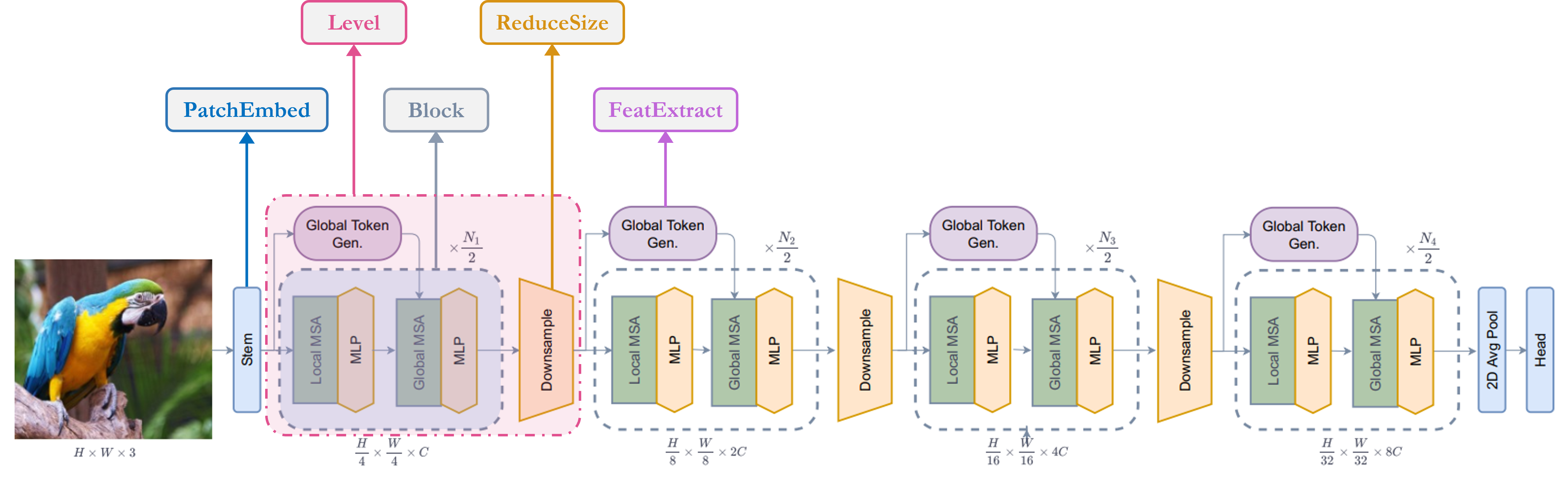

单元模块

注意：这些模块用于构建论文中的其他模块。大多数模块是从其他工作中借用或对旧工作的修改版本。

SqueezeAndExcitation：Squeeze-Excitation (SE)，又称Bottleneck 模块，充当一种通道注意力。它由AvgPooling、Dense/FullyConnected (FC)/Linear、GELU 和Sigmoid 模块组成。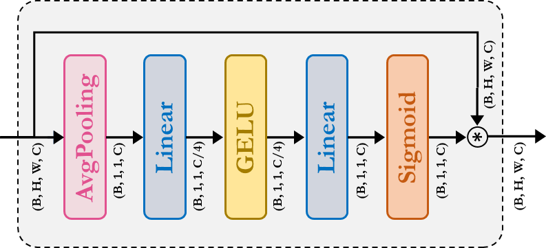
Fused-MBConv：这与 EfficientNetV2 中使用的类似。它使用Depthwise-Conv、GELU、SqueezeAndExcitation、Conv，并通过残差连接提取特征。请注意，这里没有为它声明新模块，我们只是直接应用了相应的模块。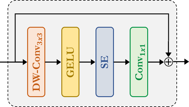
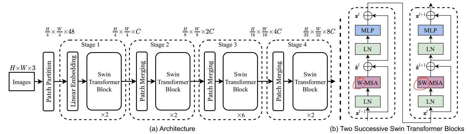
ReduceSize：这是一个基于CNN 的下采样模块，它使用上面提到的 Fused-MBConv 模块来提取特征，使用Strided Conv 同时降低空间维度和增加特征的通道维度，最后使用LayerNormalization 模块来规范化特征。在论文/图中，此模块被称为下采样模块。我认为值得一提的是，Swin Transformer 使用 PatchMerging 模块而不是 ReduceSize 来降低空间维度并增加通道维度，其中使用了全连接/密集/线性模块。根据GCViT 论文，使用 ReduceSize 的目的之一是通过CNN 模块添加归纳偏置。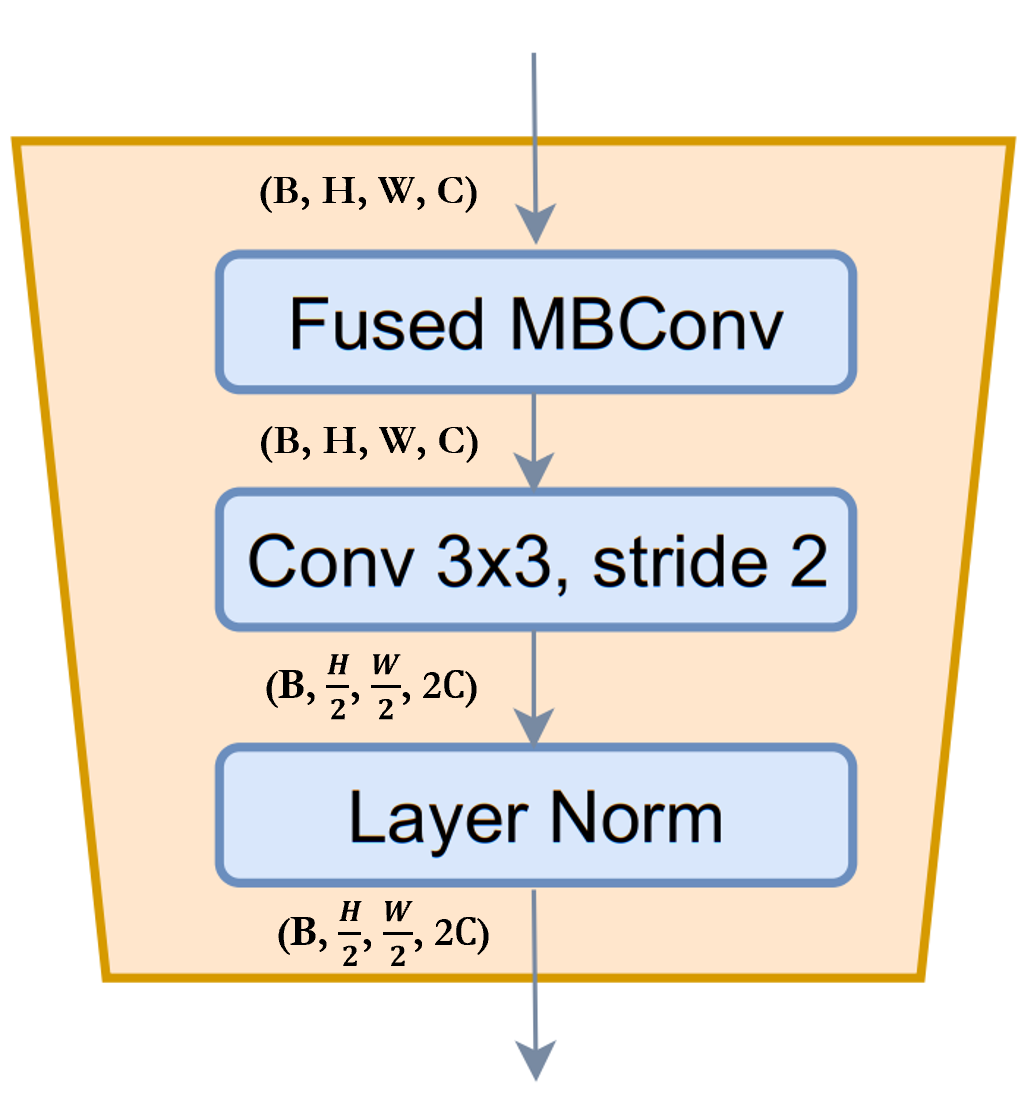
MLP：这是我们自有的多层感知机模块。这是一个前馈/全连接/线性模块，它只是将输入投影到任意维度。

class SqueezeAndExcitation(layers.Layer):
    """Squeeze and excitation block.

    Args:
        output_dim: output features dimension, if `None` use same dim as input.
        expansion: expansion ratio.
    """

    def __init__(self, output_dim=None, expansion=0.25, **kwargs):
        super().__init__(**kwargs)
        self.expansion = expansion
        self.output_dim = output_dim

    def build(self, input_shape):
        inp = input_shape[-1]
        self.output_dim = self.output_dim or inp
        self.avg_pool = layers.GlobalAvgPool2D(keepdims=True, name="avg_pool")
        self.fc = [
            layers.Dense(int(inp * self.expansion), use_bias=False, name="fc_0"),
            layers.Activation("gelu", name="fc_1"),
            layers.Dense(self.output_dim, use_bias=False, name="fc_2"),
            layers.Activation("sigmoid", name="fc_3"),
        ]
        super().build(input_shape)

    def call(self, inputs, **kwargs):
        x = self.avg_pool(inputs)
        for layer in self.fc:
            x = layer(x)
        return x * inputs


class ReduceSize(layers.Layer):
    """Down-sampling block.

    Args:
        keepdims: if False spatial dim is reduced and channel dim is increased
    """

    def __init__(self, keepdims=False, **kwargs):
        super().__init__(**kwargs)
        self.keepdims = keepdims

    def build(self, input_shape):
        embed_dim = input_shape[-1]
        dim_out = embed_dim if self.keepdims else 2 * embed_dim
        self.pad1 = layers.ZeroPadding2D(1, name="pad1")
        self.pad2 = layers.ZeroPadding2D(1, name="pad2")
        self.conv = [
            layers.DepthwiseConv2D(
                kernel_size=3, strides=1, padding="valid", use_bias=False, name="conv_0"
            ),
            layers.Activation("gelu", name="conv_1"),
            SqueezeAndExcitation(name="conv_2"),
            layers.Conv2D(
                embed_dim,
                kernel_size=1,
                strides=1,
                padding="valid",
                use_bias=False,
                name="conv_3",
            ),
        ]
        self.reduction = layers.Conv2D(
            dim_out,
            kernel_size=3,
            strides=2,
            padding="valid",
            use_bias=False,
            name="reduction",
        )
        self.norm1 = layers.LayerNormalization(
            -1, 1e-05, name="norm1"
        )  # eps like PyTorch
        self.norm2 = layers.LayerNormalization(-1, 1e-05, name="norm2")

    def call(self, inputs, **kwargs):
        x = self.norm1(inputs)
        xr = self.pad1(x)
        for layer in self.conv:
            xr = layer(xr)
        x = x + xr
        x = self.pad2(x)
        x = self.reduction(x)
        x = self.norm2(x)
        return x


class MLP(layers.Layer):
    """Multi-Layer Perceptron (MLP) block.

    Args:
        hidden_features: hidden features dimension.
        out_features: output features dimension.
        activation: activation function.
        dropout: dropout rate.
    """

    def __init__(
        self,
        hidden_features=None,
        out_features=None,
        activation="gelu",
        dropout=0.0,
        **kwargs,
    ):
        super().__init__(**kwargs)
        self.hidden_features = hidden_features
        self.out_features = out_features
        self.activation = activation
        self.dropout = dropout

    def build(self, input_shape):
        self.in_features = input_shape[-1]
        self.hidden_features = self.hidden_features or self.in_features
        self.out_features = self.out_features or self.in_features
        self.fc1 = layers.Dense(self.hidden_features, name="fc1")
        self.act = layers.Activation(self.activation, name="act")
        self.fc2 = layers.Dense(self.out_features, name="fc2")
        self.drop1 = layers.Dropout(self.dropout, name="drop1")
        self.drop2 = layers.Dropout(self.dropout, name="drop2")

    def call(self, inputs, **kwargs):
        x = self.fc1(inputs)
        x = self.act(x)
        x = self.drop1(x)
        x = self.fc2(x)
        x = self.drop2(x)
        return x

Stem

注意：在代码中，此模块被称为 PatchEmbed，但在论文中，它被称为 Stem。

在模型中，我们首先使用了 patch_embed 模块。让我们尝试理解这个模块。从 call 方法可以看出：1. 此模块首先填充输入。2. 然后使用卷积提取具有嵌入的图像块。3. 最后，使用 ReduceSize 模块先用卷积提取特征，但不降低空间维度也不增加空间维度。4. 一个重要的注意事项是，与ViT 或Swin Transformer 不同，GCViT 创建的是重叠的图像块。我们可以从代码中注意到这一点：Conv2D(self.embed_dim, kernel_size=3, strides=2, name='proj')。如果我们想要非重叠的图像块，那么我们会使用相同的 kernel_size 和 stride。5. 此模块将输入的空间维度缩小 4 倍。

总结：图像 → 填充 → 卷积 → (特征提取 + 下采样)

class PatchEmbed(layers.Layer):
    """Patch embedding block.

    Args:
        embed_dim: feature size dimension.
    """

    def __init__(self, embed_dim, **kwargs):
        super().__init__(**kwargs)
        self.embed_dim = embed_dim

    def build(self, input_shape):
        self.pad = layers.ZeroPadding2D(1, name="pad")
        self.proj = layers.Conv2D(self.embed_dim, 3, 2, name="proj")
        self.conv_down = ReduceSize(keepdims=True, name="conv_down")

    def call(self, inputs, **kwargs):
        x = self.pad(inputs)
        x = self.proj(x)
        x = self.conv_down(x)
        return x

全局 Token 生成

注意：这是用于施加归纳偏置的两个CNN 模块之一。

从上面的单元格可以看出，在 level 中，我们首先使用了 to_q_global/Global Token Gen./FeatureExtraction。让我们尝试理解它是如何工作的：

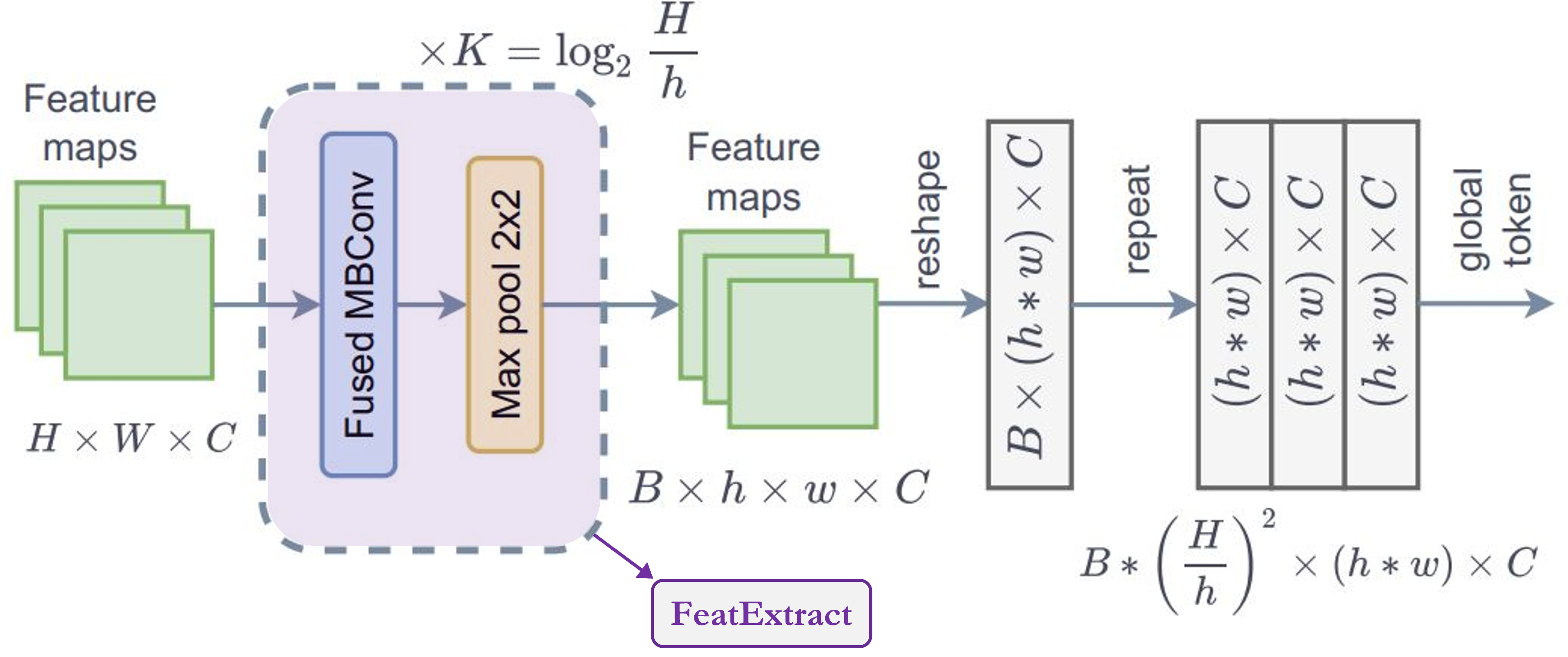
此模块是 FeatureExtract 模块的系列。根据论文，我们需要将此模块重复 K 次，其中 K = log2(H/h)，H = 特征图高度，W = 特征图宽度。
FeatureExtraction：此层与 ReduceSize 模块非常相似，除了它使用MaxPooling 模块来降低维度，它不增加特征维度（通道数），也不使用LayerNormalization。此模块用于在 Generate Token Gen. 模块中重复使用，以生成用于全局上下文注意力的全局 token。
从图中可以注意到的一个重要点是，全局 token 在整个图像中共享，这意味着我们只使用一个全局窗口来处理图像中的所有局部 token。这使得计算非常高效。
对于输入特征图，形状为 (B, H, W, C)，输出形状为 (B, h, w, C)。如果我们为图像中的总共 M 个局部窗口（其中 M = (H x W)/(h x w) = 窗口数）复制这些全局 token，那么输出形状为：(B * M, h, w, C)。

总结：此模块用于调整图像大小以适应窗口。

class FeatureExtraction(layers.Layer):
    """Feature extraction block.

    Args:
        keepdims: bool argument for maintaining the resolution.
    """

    def __init__(self, keepdims=False, **kwargs):
        super().__init__(**kwargs)
        self.keepdims = keepdims

    def build(self, input_shape):
        embed_dim = input_shape[-1]
        self.pad1 = layers.ZeroPadding2D(1, name="pad1")
        self.pad2 = layers.ZeroPadding2D(1, name="pad2")
        self.conv = [
            layers.DepthwiseConv2D(3, 1, use_bias=False, name="conv_0"),
            layers.Activation("gelu", name="conv_1"),
            SqueezeAndExcitation(name="conv_2"),
            layers.Conv2D(embed_dim, 1, 1, use_bias=False, name="conv_3"),
        ]
        if not self.keepdims:
            self.pool = layers.MaxPool2D(3, 2, name="pool")
        super().build(input_shape)

    def call(self, inputs, **kwargs):
        x = inputs
        xr = self.pad1(x)
        for layer in self.conv:
            xr = layer(xr)
        x = x + xr
        if not self.keepdims:
            x = self.pool(self.pad2(x))
        return x


class GlobalQueryGenerator(layers.Layer):
    """Global query generator.

    Args:
        keepdims: to keep the dimension of FeatureExtraction layer.
        For instance, repeating log(56/7) = 3 blocks, with input
        window dimension 56 and output window dimension 7 at down-sampling
        ratio 2. Please check Fig.5 of GC ViT paper for details.
    """

    def __init__(self, keepdims=False, **kwargs):
        super().__init__(**kwargs)
        self.keepdims = keepdims

    def build(self, input_shape):
        self.to_q_global = [
            FeatureExtraction(keepdims, name=f"to_q_global_{i}")
            for i, keepdims in enumerate(self.keepdims)
        ]
        super().build(input_shape)

    def call(self, inputs, **kwargs):
        x = inputs
        for layer in self.to_q_global:
            x = layer(x)
        return x

注意力

注意：这是论文的核心贡献。

从 call 方法可以看出：1. WindowAttention 模块根据 global_query 参数应用局部和全局窗口注意力。

首先，它将输入特征转换为局部注意力的 query、key、value 和全局注意力的 key、value。对于全局注意力，它从 Global Token Gen. 获取全局查询。代码中一个值得注意的地方是，我们将特征或 embed_dim 分配给Transformer 的所有头以减少计算量。qkv = tf.reshape(qkv, [B_, N, self.qkv_size, self.num_heads, C // self.num_heads])
在将查询、键和值发送用于注意力之前，全局 token 会经历一个重要过程。相同的全局 token 或一个全局窗口会被复制到所有局部窗口以提高效率。q_global = tf.repeat(q_global, repeats=B_//B, axis=0)，这里 B_//B 表示图像中的窗口数。
然后，根据 global_query 参数，简单地应用局部窗口自注意力或全局窗口注意力。代码中值得注意的一点是，我们将相对位置嵌入添加到注意力掩码而不是图像块嵌入。attn = attn + relative_position_bias[tf.newaxis,]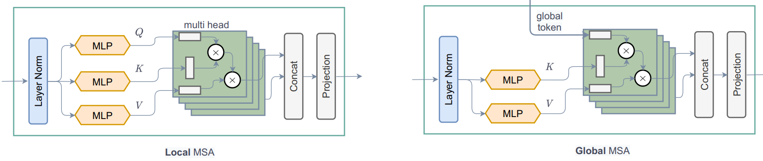
现在，让我们思考一下并尝试理解这里发生的事情。让我们关注下面的图。从左侧可以看出，在局部注意力中，查询是局部的，并且仅限于局部窗口（红色方框边框），因此我们无法获得长距离信息。但在右侧，由于全局查询，我们现在不受限于局部窗口（蓝色方框边框），并且可以获得长距离信息。
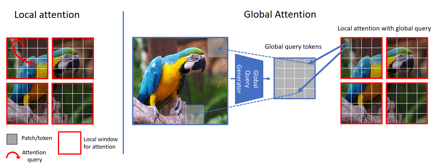
在 ViT 中，我们将图像 token 与图像 token 进行比较（注意力），在 Swin Transformer 中，我们将窗口 token 与窗口 token 进行比较，但在 GCViT 中，我们将图像 token 与窗口 token 进行比较。但是现在你可能会问，即使图像 token 的尺寸比窗口 token 大，我们如何比较（注意力）图像 token 和窗口 token 呢？（从上面的图中，图像 token 的形状为 (1, 8, 8, 3)，窗口 token 的形状为 (1, 4, 4, 3)）。是的，你说得对，我们不能直接比较它们，因此我们使用 Global Token Gen./FeatureExtraction CNN 模块将图像 token 调整大小以匹配窗口 token。下表应能清晰地比较：

模型	查询 Token	键-值 Token	注意力类型	注意力覆盖范围
ViT	图像	图像	自注意力	全局
Swin Transformer	窗口	窗口	自注意力	局部
GCViT	调整大小后的图像	窗口	图像-窗口注意力	全局

class WindowAttention(layers.Layer):
    """Local window attention.

    This implementation was proposed by
    [Liu et al., 2021](https://arxiv.org/abs/2103.14030) in SwinTransformer.

    Args:
        window_size: window size.
        num_heads: number of attention head.
        global_query: if the input contains global_query
        qkv_bias: bool argument for query, key, value learnable bias.
        qk_scale: bool argument to scaling query, key.
        attention_dropout: attention dropout rate.
        projection_dropout: output dropout rate.
    """

    def __init__(
        self,
        window_size,
        num_heads,
        global_query,
        qkv_bias=True,
        qk_scale=None,
        attention_dropout=0.0,
        projection_dropout=0.0,
        **kwargs,
    ):
        super().__init__(**kwargs)
        window_size = (window_size, window_size)
        self.window_size = window_size
        self.num_heads = num_heads
        self.global_query = global_query
        self.qkv_bias = qkv_bias
        self.qk_scale = qk_scale
        self.attention_dropout = attention_dropout
        self.projection_dropout = projection_dropout

    def build(self, input_shape):
        embed_dim = input_shape[0][-1]
        head_dim = embed_dim // self.num_heads
        self.scale = self.qk_scale or head_dim**-0.5
        self.qkv_size = 3 - int(self.global_query)
        self.qkv = layers.Dense(
            embed_dim * self.qkv_size, use_bias=self.qkv_bias, name="qkv"
        )
        self.relative_position_bias_table = self.add_weight(
            name="relative_position_bias_table",
            shape=[
                (2 * self.window_size[0] - 1) * (2 * self.window_size[1] - 1),
                self.num_heads,
            ],
            initializer=keras.initializers.TruncatedNormal(stddev=0.02),
            trainable=True,
            dtype=self.dtype,
        )
        self.attn_drop = layers.Dropout(self.attention_dropout, name="attn_drop")
        self.proj = layers.Dense(embed_dim, name="proj")
        self.proj_drop = layers.Dropout(self.projection_dropout, name="proj_drop")
        self.softmax = layers.Activation("softmax", name="softmax")
        super().build(input_shape)

    def get_relative_position_index(self):
        coords_h = ops.arange(self.window_size[0])
        coords_w = ops.arange(self.window_size[1])
        coords = ops.stack(ops.meshgrid(coords_h, coords_w, indexing="ij"), axis=0)
        coords_flatten = ops.reshape(coords, [2, -1])
        relative_coords = coords_flatten[:, :, None] - coords_flatten[:, None, :]
        relative_coords = ops.transpose(relative_coords, axes=[1, 2, 0])
        relative_coords_xx = relative_coords[:, :, 0] + self.window_size[0] - 1
        relative_coords_yy = relative_coords[:, :, 1] + self.window_size[1] - 1
        relative_coords_xx = relative_coords_xx * (2 * self.window_size[1] - 1)
        relative_position_index = relative_coords_xx + relative_coords_yy
        return relative_position_index

    def call(self, inputs, **kwargs):
        if self.global_query:
            inputs, q_global = inputs
            B = ops.shape(q_global)[0]  # B, N, C
        else:
            inputs = inputs[0]
        B_, N, C = ops.shape(inputs)  # B*num_window, num_tokens, channels
        qkv = self.qkv(inputs)
        qkv = ops.reshape(
            qkv, [B_, N, self.qkv_size, self.num_heads, C // self.num_heads]
        )
        qkv = ops.transpose(qkv, [2, 0, 3, 1, 4])
        if self.global_query:
            k, v = ops.split(
                qkv, indices_or_sections=2, axis=0
            )  # for unknown shame num=None will throw error
            q_global = ops.repeat(
                q_global, repeats=B_ // B, axis=0
            )  # num_windows = B_//B => q_global same for all windows in a img
            q = ops.reshape(q_global, [B_, N, self.num_heads, C // self.num_heads])
            q = ops.transpose(q, axes=[0, 2, 1, 3])
        else:
            q, k, v = ops.split(qkv, indices_or_sections=3, axis=0)
            q = ops.squeeze(q, axis=0)

        k = ops.squeeze(k, axis=0)
        v = ops.squeeze(v, axis=0)

        q = q * self.scale
        attn = q @ ops.transpose(k, axes=[0, 1, 3, 2])
        relative_position_bias = ops.take(
            self.relative_position_bias_table,
            ops.reshape(self.get_relative_position_index(), [-1]),
        )
        relative_position_bias = ops.reshape(
            relative_position_bias,
            [
                self.window_size[0] * self.window_size[1],
                self.window_size[0] * self.window_size[1],
                -1,
            ],
        )
        relative_position_bias = ops.transpose(relative_position_bias, axes=[2, 0, 1])
        attn = attn + relative_position_bias[None,]
        attn = self.softmax(attn)
        attn = self.attn_drop(attn)

        x = ops.transpose((attn @ v), axes=[0, 2, 1, 3])
        x = ops.reshape(x, [B_, N, C])
        x = self.proj_drop(self.proj(x))
        return x

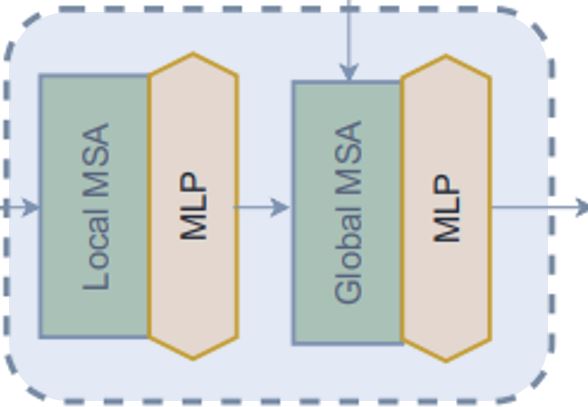
Block

注意：此模块不包含任何卷积模块。

在 level 中，第二个模块是 block。让我们尝试理解它是如何工作的。从 call 方法可以看出：1. Block 模块仅接受特征图以进行局部注意力，或者接受额外的全局查询以进行全局注意力。2. 在将特征图发送用于注意力之前，此模块将批处理特征图转换为批处理窗口，因为我们将应用窗口注意力。3. 然后我们将批处理批处理窗口发送用于注意力。4. 应用注意力后，我们将批处理窗口还原为批处理特征图。5. 在将注意力应用于的特征输出之前，此模块在残差连接中应用随机深度正则化。另外，在应用随机深度之前，它会使用可训练参数对输入进行缩放。请注意，此随机深度块未在论文的图中显示。

窗口

在 block 模块中，我们在应用注意力之前和之后创建了窗口。让我们尝试理解我们是如何创建窗口的：* 以下模块将特征图 (B, H, W, C) 转换为堆叠窗口 (B x H/h x W/w, h, w, C) → (窗口批次数, 窗口大小, 窗口大小, 通道数) * 此模块使用 reshape 和 transpose 来从图像创建这些窗口，而不是迭代它们。

class Block(layers.Layer):
    """GCViT block.

    Args:
        window_size: window size.
        num_heads: number of attention head.
        global_query: apply global window attention
        mlp_ratio: MLP ratio.
        qkv_bias: bool argument for query, key, value learnable bias.
        qk_scale: bool argument to scaling query, key.
        drop: dropout rate.
        attention_dropout: attention dropout rate.
        path_drop: drop path rate.
        activation: activation function.
        layer_scale: layer scaling coefficient.
    """

    def __init__(
        self,
        window_size,
        num_heads,
        global_query,
        mlp_ratio=4.0,
        qkv_bias=True,
        qk_scale=None,
        dropout=0.0,
        attention_dropout=0.0,
        path_drop=0.0,
        activation="gelu",
        layer_scale=None,
        **kwargs,
    ):
        super().__init__(**kwargs)
        self.window_size = window_size
        self.num_heads = num_heads
        self.global_query = global_query
        self.mlp_ratio = mlp_ratio
        self.qkv_bias = qkv_bias
        self.qk_scale = qk_scale
        self.dropout = dropout
        self.attention_dropout = attention_dropout
        self.path_drop = path_drop
        self.activation = activation
        self.layer_scale = layer_scale

    def build(self, input_shape):
        B, H, W, C = input_shape[0]
        self.norm1 = layers.LayerNormalization(-1, 1e-05, name="norm1")
        self.attn = WindowAttention(
            window_size=self.window_size,
            num_heads=self.num_heads,
            global_query=self.global_query,
            qkv_bias=self.qkv_bias,
            qk_scale=self.qk_scale,
            attention_dropout=self.attention_dropout,
            projection_dropout=self.dropout,
            name="attn",
        )
        self.drop_path1 = DropPath(self.path_drop)
        self.drop_path2 = DropPath(self.path_drop)
        self.norm2 = layers.LayerNormalization(-1, 1e-05, name="norm2")
        self.mlp = MLP(
            hidden_features=int(C * self.mlp_ratio),
            dropout=self.dropout,
            activation=self.activation,
            name="mlp",
        )
        if self.layer_scale is not None:
            self.gamma1 = self.add_weight(
                name="gamma1",
                shape=[C],
                initializer=keras.initializers.Constant(self.layer_scale),
                trainable=True,
                dtype=self.dtype,
            )
            self.gamma2 = self.add_weight(
                name="gamma2",
                shape=[C],
                initializer=keras.initializers.Constant(self.layer_scale),
                trainable=True,
                dtype=self.dtype,
            )
        else:
            self.gamma1 = 1.0
            self.gamma2 = 1.0
        self.num_windows = int(H // self.window_size) * int(W // self.window_size)
        super().build(input_shape)

    def call(self, inputs, **kwargs):
        if self.global_query:
            inputs, q_global = inputs
        else:
            inputs = inputs[0]
        B, H, W, C = ops.shape(inputs)
        x = self.norm1(inputs)
        # create windows and concat them in batch axis
        x = self.window_partition(x, self.window_size)  # (B_, win_h, win_w, C)
        # flatten patch
        x = ops.reshape(x, [-1, self.window_size * self.window_size, C])
        # attention
        if self.global_query:
            x = self.attn([x, q_global])
        else:
            x = self.attn([x])
        # reverse window partition
        x = self.window_reverse(x, self.window_size, H, W, C)
        # FFN
        x = inputs + self.drop_path1(x * self.gamma1)
        x = x + self.drop_path2(self.gamma2 * self.mlp(self.norm2(x)))
        return x

    def window_partition(self, x, window_size):
        """
        Args:
            x: (B, H, W, C)
            window_size: window size
        Returns:
            local window features (num_windows*B, window_size, window_size, C)
        """
        B, H, W, C = ops.shape(x)
        x = ops.reshape(
            x,
            [
                -1,
                H // window_size,
                window_size,
                W // window_size,
                window_size,
                C,
            ],
        )
        x = ops.transpose(x, axes=[0, 1, 3, 2, 4, 5])
        windows = ops.reshape(x, [-1, window_size, window_size, C])
        return windows

    def window_reverse(self, windows, window_size, H, W, C):
        """
        Args:
            windows: local window features (num_windows*B, window_size, window_size, C)
            window_size: Window size
            H: Height of image
            W: Width of image
            C: Channel of image
        Returns:
            x: (B, H, W, C)
        """
        x = ops.reshape(
            windows,
            [
                -1,
                H // window_size,
                W // window_size,
                window_size,
                window_size,
                C,
            ],
        )
        x = ops.transpose(x, axes=[0, 1, 3, 2, 4, 5])
        x = ops.reshape(x, [-1, H, W, C])
        return x

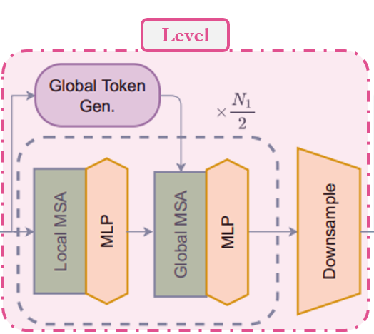
Level

注意：此模块同时包含 Transformer 和 CNN 模块。

在模型中，我们使用的第二个模块是 level。让我们尝试理解这个模块。从 call 方法可以看出：1. 首先，它使用一系列 FeatureExtraction 模块创建全局 token。我们稍后会看到 FeatureExtraction 只是一个简单的CNN 模块。2. 然后，它使用一系列 Block 模块，根据深度级别应用局部或全局窗口注意力。3. 最后，它使用 ReduceSize 来降低上下文特征的维度。

总结：特征图 → 全局 token → 局部/全局窗口注意力 → 下采样

class Level(layers.Layer):
    """GCViT level.

    Args:
        depth: number of layers in each stage.
        num_heads: number of heads in each stage.
        window_size: window size in each stage.
        keepdims: dims to keep in FeatureExtraction.
        downsample: bool argument for down-sampling.
        mlp_ratio: MLP ratio.
        qkv_bias: bool argument for query, key, value learnable bias.
        qk_scale: bool argument to scaling query, key.
        drop: dropout rate.
        attention_dropout: attention dropout rate.
        path_drop: drop path rate.
        layer_scale: layer scaling coefficient.
    """

    def __init__(
        self,
        depth,
        num_heads,
        window_size,
        keepdims,
        downsample=True,
        mlp_ratio=4.0,
        qkv_bias=True,
        qk_scale=None,
        dropout=0.0,
        attention_dropout=0.0,
        path_drop=0.0,
        layer_scale=None,
        **kwargs,
    ):
        super().__init__(**kwargs)
        self.depth = depth
        self.num_heads = num_heads
        self.window_size = window_size
        self.keepdims = keepdims
        self.downsample = downsample
        self.mlp_ratio = mlp_ratio
        self.qkv_bias = qkv_bias
        self.qk_scale = qk_scale
        self.dropout = dropout
        self.attention_dropout = attention_dropout
        self.path_drop = path_drop
        self.layer_scale = layer_scale

    def build(self, input_shape):
        path_drop = (
            [self.path_drop] * self.depth
            if not isinstance(self.path_drop, list)
            else self.path_drop
        )
        self.blocks = [
            Block(
                window_size=self.window_size,
                num_heads=self.num_heads,
                global_query=bool(i % 2),
                mlp_ratio=self.mlp_ratio,
                qkv_bias=self.qkv_bias,
                qk_scale=self.qk_scale,
                dropout=self.dropout,
                attention_dropout=self.attention_dropout,
                path_drop=path_drop[i],
                layer_scale=self.layer_scale,
                name=f"blocks_{i}",
            )
            for i in range(self.depth)
        ]
        self.down = ReduceSize(keepdims=False, name="downsample")
        self.q_global_gen = GlobalQueryGenerator(self.keepdims, name="q_global_gen")
        super().build(input_shape)

    def call(self, inputs, **kwargs):
        x = inputs
        q_global = self.q_global_gen(x)  # shape: (B, win_size, win_size, C)
        for i, blk in enumerate(self.blocks):
            if i % 2:
                x = blk([x, q_global])  # shape: (B, H, W, C)
            else:
                x = blk([x])  # shape: (B, H, W, C)
        if self.downsample:
            x = self.down(x)  # shape: (B, H//2, W//2, 2*C)
        return x

模型

让我们直接跳到模型。从 call 方法可以看出：1. 它从图像创建图像块嵌入。此层不会展平这些嵌入，这意味着此模块的输出将是 (batch, height/window_size, width/window_size, embed_dim) 而不是 (batch, height x width/window_size^2, embed_dim)。2. 然后它应用 Dropout 模块，该模块会随机将输入单元设置为 0。3. 它将这些嵌入传递给一系列 Level 模块，我们称之为 level，其中：1. 全局 token 被生成 1. 应用局部和全局注意力 1. 最后应用下采样。4. 因此，经过 n 个级别后的输出形状为：(batch, width/window_size x 2^{n-1}, width/window_size x 2^{n-1}, embed_dim x 2^{n-1})。在最后一层，论文不使用下采样并增加通道数。5. 上层输出使用 LayerNormalization 模块进行规范化。6. 在 head 中，2D 特征通过 Pooling 模块转换为 1D 特征。此模块后的输出形状为 (batch, embed_dim x 2^{n-1})。7. 最后，将池化后的特征送入 Dense/Linear 模块进行分类。

总结：图像 → (图像块 + 嵌入) → Dropout → (注意力 + 特征提取) → 规范化 → 池化 → 分类

class GCViT(keras.Model):
    """GCViT model.

    Args:
        window_size: window size in each stage.
        embed_dim: feature size dimension.
        depths: number of layers in each stage.
        num_heads: number of heads in each stage.
        drop_rate: dropout rate.
        mlp_ratio: MLP ratio.
        qkv_bias: bool argument for query, key, value learnable bias.
        qk_scale: bool argument to scaling query, key.
        attention_dropout: attention dropout rate.
        path_drop: drop path rate.
        layer_scale: layer scaling coefficient.
        num_classes: number of classes.
        head_activation: activation function for head.
    """

    def __init__(
        self,
        window_size,
        embed_dim,
        depths,
        num_heads,
        drop_rate=0.0,
        mlp_ratio=3.0,
        qkv_bias=True,
        qk_scale=None,
        attention_dropout=0.0,
        path_drop=0.1,
        layer_scale=None,
        num_classes=1000,
        head_activation="softmax",
        **kwargs,
    ):
        super().__init__(**kwargs)
        self.window_size = window_size
        self.embed_dim = embed_dim
        self.depths = depths
        self.num_heads = num_heads
        self.drop_rate = drop_rate
        self.mlp_ratio = mlp_ratio
        self.qkv_bias = qkv_bias
        self.qk_scale = qk_scale
        self.attention_dropout = attention_dropout
        self.path_drop = path_drop
        self.layer_scale = layer_scale
        self.num_classes = num_classes
        self.head_activation = head_activation

        self.patch_embed = PatchEmbed(embed_dim=embed_dim, name="patch_embed")
        self.pos_drop = layers.Dropout(drop_rate, name="pos_drop")
        path_drops = np.linspace(0.0, path_drop, sum(depths))
        keepdims = [(0, 0, 0), (0, 0), (1,), (1,)]
        self.levels = []
        for i in range(len(depths)):
            path_drop = path_drops[sum(depths[:i]) : sum(depths[: i + 1])].tolist()
            level = Level(
                depth=depths[i],
                num_heads=num_heads[i],
                window_size=window_size[i],
                keepdims=keepdims[i],
                downsample=(i < len(depths) - 1),
                mlp_ratio=mlp_ratio,
                qkv_bias=qkv_bias,
                qk_scale=qk_scale,
                dropout=drop_rate,
                attention_dropout=attention_dropout,
                path_drop=path_drop,
                layer_scale=layer_scale,
                name=f"levels_{i}",
            )
            self.levels.append(level)
        self.norm = layers.LayerNormalization(axis=-1, epsilon=1e-05, name="norm")
        self.pool = layers.GlobalAvgPool2D(name="pool")
        self.head = layers.Dense(num_classes, name="head", activation=head_activation)

    def build(self, input_shape):
        super().build(input_shape)
        self.built = True

    def call(self, inputs, **kwargs):
        x = self.patch_embed(inputs)  # shape: (B, H, W, C)
        x = self.pos_drop(x)
        for level in self.levels:
            x = level(x)  # shape: (B, H_, W_, C_)
        x = self.norm(x)
        x = self.pool(x)  # shape: (B, C__)
        x = self.head(x)
        return x

    def build_graph(self, input_shape=(224, 224, 3)):
        """
        ref: https://www.kaggle.com/code/ipythonx/tf-hybrid-efficientnet-swin-transformer-gradcam
        """
        x = keras.Input(shape=input_shape)
        return keras.Model(inputs=[x], outputs=self.call(x), name=self.name)

    def summary(self, input_shape=(224, 224, 3)):
        return self.build_graph(input_shape).summary()

构建模型

让我们使用上面解释的所有模块来构建一个完整的模型。我们将构建 GCViT-XXTiny 模型，并使用论文中提到的配置。
我们还将加载移植的官方预训练权重，并尝试进行一些预测。

# Model Configs
config = {
    "window_size": (7, 7, 14, 7),
    "embed_dim": 64,
    "depths": (2, 2, 6, 2),
    "num_heads": (2, 4, 8, 16),
    "mlp_ratio": 3.0,
    "path_drop": 0.2,
}
ckpt_link = (
    "https://github.com/awsaf49/gcvit-tf/releases/download/v1.1.6/gcvitxxtiny.keras"
)

# Build Model
model = GCViT(**config)
inp = ops.array(np.random.uniform(size=(1, 224, 224, 3)))
out = model(inp)

# Load Weights
ckpt_path = keras.utils.get_file(ckpt_link.split("/")[-1], ckpt_link)
model.load_weights(ckpt_path)

# Summary
model.summary((224, 224, 3))

Downloading data from https://github.com/awsaf49/gcvit-tf/releases/download/v1.1.6/gcvitxxtiny.keras
 48767519/48767519 ━━━━━━━━━━━━━━━━━━━━ 0s 0us/step

Model: "gc_vi_t"

┏━━━━━━━━━━━━━━━━━━━━━━━━━━━━━━━━━━━━┳━━━━━━━━━━━━━━━━━━━━━━━━━━━━━━━┳━━━━━━━━━━━━━┓
┃ Layer (type)                       ┃ Output Shape                  ┃     Param # ┃
┡━━━━━━━━━━━━━━━━━━━━━━━━━━━━━━━━━━━━╇━━━━━━━━━━━━━━━━━━━━━━━━━━━━━━━╇━━━━━━━━━━━━━┩
│ input_layer (InputLayer)           │ (None, 224, 224, 3)           │           0 │
├────────────────────────────────────┼───────────────────────────────┼─────────────┤
│ patch_embed (PatchEmbed)           │ (None, 56, 56, 64)            │      45,632 │
├────────────────────────────────────┼───────────────────────────────┼─────────────┤
│ pos_drop (Dropout)                 │ (None, 56, 56, 64)            │           0 │
├────────────────────────────────────┼───────────────────────────────┼─────────────┤
│ levels_0 (Level)                   │ (None, 28, 28, 128)           │     180,964 │
├────────────────────────────────────┼───────────────────────────────┼─────────────┤
│ levels_1 (Level)                   │ (None, 14, 14, 256)           │     688,456 │
├────────────────────────────────────┼───────────────────────────────┼─────────────┤
│ levels_2 (Level)                   │ (None, 7, 7, 512)             │   5,170,608 │
├────────────────────────────────────┼───────────────────────────────┼─────────────┤
│ levels_3 (Level)                   │ (None, 7, 7, 512)             │   5,395,744 │
├────────────────────────────────────┼───────────────────────────────┼─────────────┤
│ norm (LayerNormalization)          │ (None, 7, 7, 512)             │       1,024 │
├────────────────────────────────────┼───────────────────────────────┼─────────────┤
│ pool (GlobalAveragePooling2D)      │ (None, 512)                   │           0 │
├────────────────────────────────────┼───────────────────────────────┼─────────────┤
│ head (Dense)                       │ (None, 1000)                  │     513,000 │
└────────────────────────────────────┴───────────────────────────────┴─────────────┘

 Total params: 11,995,428 (45.76 MB)

 Trainable params: 11,995,428 (45.76 MB)

 Non-trainable params: 0 (0.00 B)

预训练权重健全性检查

img = keras.applications.imagenet_utils.preprocess_input(
    chelsea(), mode="torch"
)  # Chelsea the cat
img = ops.image.resize(img, (224, 224))[None,]  # resize & create batch
pred = model(img)
pred_dec = keras.applications.imagenet_utils.decode_predictions(pred)[0]

print("\n# Image:")
plt.figure(figsize=(6, 6))
plt.imshow(chelsea())
plt.show()
print()

print("# Prediction (Top 5):")
for i in range(5):
    print("{:<12} : {:0.2f}".format(pred_dec[i][1], pred_dec[i][2]))

Downloading data from https://storage.googleapis.com/download.tensorflow.org/data/imagenet_class_index.json
 35363/35363 ━━━━━━━━━━━━━━━━━━━━ 0s 0us/step

# Image:

png

# Prediction (Top 5):
Egyptian_cat : 0.72
tiger_cat    : 0.04
tabby        : 0.03
crossword_puzzle : 0.01
panpipe      : 0.00

微调 GCViT 模型

在接下来的单元格中，我们将使用包含 104 个类别的 Flower 数据集对 GCViT 模型进行微调。

配置

# Model
IMAGE_SIZE = (224, 224)

# Hyper Params
BATCH_SIZE = 32
EPOCHS = 5

# Dataset
CLASSES = [
    "dandelion",
    "daisy",
    "tulips",
    "sunflowers",
    "roses",
]  # don't change the order

# Other constants
MEAN = 255 * np.array([0.485, 0.456, 0.406], dtype="float32")  # imagenet mean
STD = 255 * np.array([0.229, 0.224, 0.225], dtype="float32")  # imagenet std
AUTO = tf.data.AUTOTUNE

数据加载器

def make_dataset(dataset: tf.data.Dataset, train: bool, image_size: int = IMAGE_SIZE):
    def preprocess(image, label):
        # for training, do augmentation
        if train:
            if tf.random.uniform(shape=[]) > 0.5:
                image = tf.image.flip_left_right(image)
        image = tf.image.resize(image, size=image_size, method="bicubic")
        image = (image - MEAN) / STD  # normalization
        return image, label

    if train:
        dataset = dataset.shuffle(BATCH_SIZE * 10)

    return dataset.map(preprocess, AUTO).batch(BATCH_SIZE).prefetch(AUTO)

Flower 数据集

train_dataset, val_dataset = tfds.load(
    "tf_flowers",
    split=["train[:90%]", "train[90%:]"],
    as_supervised=True,
    try_gcs=False,  # gcs_path is necessary for tpu,
)

train_dataset = make_dataset(train_dataset, True)
val_dataset = make_dataset(val_dataset, False)

Downloading and preparing dataset 218.21 MiB (download: 218.21 MiB, generated: 221.83 MiB, total: 440.05 MiB) to /root/tensorflow_datasets/tf_flowers/3.0.1...

Dl Completed...:   0%|          | 0/5 [00:00<?, ? file/s]

Dataset tf_flowers downloaded and prepared to /root/tensorflow_datasets/tf_flowers/3.0.1. Subsequent calls will reuse this data.

为 Flower 数据集重新构建模型

# Re-Build Model
model = GCViT(**config, num_classes=104)
inp = ops.array(np.random.uniform(size=(1, 224, 224, 3)))
out = model(inp)

# Load Weights
ckpt_path = keras.utils.get_file(ckpt_link.split("/")[-1], ckpt_link)
model.load_weights(ckpt_path, skip_mismatch=True)

model.compile(
    loss="sparse_categorical_crossentropy", optimizer="adam", metrics=["accuracy"]
)

/usr/local/lib/python3.10/dist-packages/keras/src/saving/saving_lib.py:269: UserWarning: A total of 1 objects could not be loaded. Example error message for object <Dense name=head, built=True>:

Layer 'head' expected 2 variables, but received 0 variables during loading. Expected: ['kernel', 'bias']

List of objects that could not be loaded:
[<Dense name=head, built=True>]
  warnings.warn(msg)

训练

history = model.fit(
    train_dataset, validation_data=val_dataset, epochs=EPOCHS, verbose=1
)

Epoch 1/5
 104/104 ━━━━━━━━━━━━━━━━━━━━ 153s 581ms/step - accuracy: 0.5140 - loss: 1.4615 - val_accuracy: 0.8828 - val_loss: 0.3485
Epoch 2/5
 104/104 ━━━━━━━━━━━━━━━━━━━━ 7s 69ms/step - accuracy: 0.8775 - loss: 0.3437 - val_accuracy: 0.8828 - val_loss: 0.3508
Epoch 3/5
 104/104 ━━━━━━━━━━━━━━━━━━━━ 7s 68ms/step - accuracy: 0.8937 - loss: 0.2918 - val_accuracy: 0.9019 - val_loss: 0.2953
Epoch 4/5
 104/104 ━━━━━━━━━━━━━━━━━━━━ 7s 68ms/step - accuracy: 0.9232 - loss: 0.2397 - val_accuracy: 0.9183 - val_loss: 0.2212
Epoch 5/5
 104/104 ━━━━━━━━━━━━━━━━━━━━ 7s 68ms/step - accuracy: 0.9456 - loss: 0.1645 - val_accuracy: 0.9210 - val_loss: 0.2897