手写体识别
作者: A_K_Nain, Sayak Paul
创建日期 2021/08/16
最后修改日期 2025/09/29
描述: 训练一个具有可变长度序列的手写体识别模型。

简介
本示例展示了如何将 Captcha OCR 示例扩展到 IAM 数据集,该数据集具有可变长度的真实目标。数据集中的每个样本都是一张手写文本图像,其对应的目标是图像中存在的字符串。IAM 数据集广泛用于许多 OCR 基准测试,因此我们希望本示例能为构建 OCR 系统提供一个良好的起点。
数据收集
!wget -q https://github.com/sayakpaul/Handwriting-Recognizer-in-Keras/releases/download/v1.0.0/IAM_Words.zip
!unzip -qq IAM_Words.zip
!
!mkdir data
!mkdir data/words
!tar -xf IAM_Words/words.tgz -C data/words
!mv IAM_Words/words.txt data
预览数据集的组织方式。以“#”开头的行仅为元数据信息。
!head -20 data/words.txt
#--- words.txt ---------------------------------------------------------------#
#
# iam database word information
#
# format: a01-000u-00-00 ok 154 1 408 768 27 51 AT A
#
#     a01-000u-00-00  -> word id for line 00 in form a01-000u
#     ok              -> result of word segmentation
#                            ok: word was correctly
#                            er: segmentation of word can be bad
#
#     154             -> graylevel to binarize the line containing this word
#     1               -> number of components for this word
#     408 768 27 51   -> bounding box around this word in x,y,w,h format
#     AT              -> the grammatical tag for this word, see the
#                        file tagset.txt for an explanation
#     A               -> the transcription for this word
#
a01-000u-00-00 ok 154 408 768 27 51 AT A
a01-000u-00-01 ok 154 507 766 213 48 NN MOVE
导入
import keras
from keras.layers import StringLookup
from keras import ops
import matplotlib.pyplot as plt
import tensorflow as tf
import numpy as np
import os

np.random.seed(42)
keras.utils.set_random_seed(42)
数据集划分
base_path = "data"
words_list = []

words = open(f"{base_path}/words.txt", "r").readlines()
for line in words:
    if line[0] == "#":
        continue
    if line.split(" ")[1] != "err":  # We don't need to deal with errored entries.
        words_list.append(line)

len(words_list)

np.random.shuffle(words_list)
我们将数据集按 90:5:5 的比例(训练:验证:测试)划分为三个子集。
split_idx = int(0.9 * len(words_list))
train_samples = words_list[:split_idx]
test_samples = words_list[split_idx:]

val_split_idx = int(0.5 * len(test_samples))
validation_samples = test_samples[:val_split_idx]
test_samples = test_samples[val_split_idx:]

assert len(words_list) == len(train_samples) + len(validation_samples) + len(
    test_samples
)

print(f"Total training samples: {len(train_samples)}")
print(f"Total validation samples: {len(validation_samples)}")
print(f"Total test samples: {len(test_samples)}")
Total training samples: 86810
Total validation samples: 4823
Total test samples: 4823
数据输入管道
我们首先准备图像路径,从而开始构建数据输入管道。
base_image_path = os.path.join(base_path, "words")


def get_image_paths_and_labels(samples):
    paths = []
    corrected_samples = []
    for i, file_line in enumerate(samples):
        line_split = file_line.strip()
        line_split = line_split.split(" ")

        # Each line split will have this format for the corresponding image:
        # part1/part1-part2/part1-part2-part3.png
        image_name = line_split[0]
        partI = image_name.split("-")[0]
        partII = image_name.split("-")[1]
        img_path = os.path.join(
            base_image_path, partI, partI + "-" + partII, image_name + ".png"
        )
        if os.path.getsize(img_path):
            paths.append(img_path)
            corrected_samples.append(file_line.split("\n")[0])

    return paths, corrected_samples


train_img_paths, train_labels = get_image_paths_and_labels(train_samples)
validation_img_paths, validation_labels = get_image_paths_and_labels(validation_samples)
test_img_paths, test_labels = get_image_paths_and_labels(test_samples)
然后我们准备真实标签。
# Find maximum length and the size of the vocabulary in the training data.
train_labels_cleaned = []
characters = set()
max_len = 0

for label in train_labels:
    label = label.split(" ")[-1].strip()
    for char in label:
        characters.add(char)

    max_len = max(max_len, len(label))
    train_labels_cleaned.append(label)

characters = sorted(list(characters))

print("Maximum length: ", max_len)
print("Vocab size: ", len(characters))

# Check some label samples.
train_labels_cleaned[:10]
Maximum length:  21
Vocab size:  78

['sure',
 'he',
 'during',
 'of',
 'booty',
 'gastronomy',
 'boy',
 'The',
 'and',
 'in']
现在我们也清理验证集和测试集的标签。
def clean_labels(labels):
    cleaned_labels = []
    for label in labels:
        label = label.split(" ")[-1].strip()
        cleaned_labels.append(label)
    return cleaned_labels


validation_labels_cleaned = clean_labels(validation_labels)
test_labels_cleaned = clean_labels(test_labels)
构建字符词汇表
Keras 提供了不同的预处理层来处理不同类型的数据。 本指南提供了全面的介绍。我们的示例涉及字符级别的标签预处理。这意味着,如果存在两个标签,例如“cat”和“dog”,那么我们的字符词汇表应为 {a, c, d, g, o, t}(不包含任何特殊标记)。我们为此目的使用了 StringLookup 层。
AUTOTUNE = tf.data.AUTOTUNE

# Mapping characters to integers.
char_to_num = StringLookup(vocabulary=list(characters), mask_token=None)

# Mapping integers back to original characters.
num_to_char = StringLookup(
    vocabulary=char_to_num.get_vocabulary(), mask_token=None, invert=True
)
在不失真的情况下调整图像大小
许多 OCR 模型使用矩形图像而不是方形图像。稍后当我们可视化数据集中的一些样本时,这一点会变得更加清晰。虽然不考虑长宽比调整方形图像不会引入显著的失真,但对于矩形图像则不然。但是,将图像调整为统一大小是小批量处理的要求。因此,我们需要执行调整大小操作,以满足以下标准:
- 保留长宽比。
- 图像内容不受影响。
def distortion_free_resize(image, img_size):
    w, h = img_size
    image = tf.image.resize(image, size=(h, w), preserve_aspect_ratio=True)

    # Check tha amount of padding needed to be done.
    pad_height = h - ops.shape(image)[0]
    pad_width = w - ops.shape(image)[1]

    # Only necessary if you want to do same amount of padding on both sides.
    if pad_height % 2 != 0:
        height = pad_height // 2
        pad_height_top = height + 1
        pad_height_bottom = height
    else:
        pad_height_top = pad_height_bottom = pad_height // 2

    if pad_width % 2 != 0:
        width = pad_width // 2
        pad_width_left = width + 1
        pad_width_right = width
    else:
        pad_width_left = pad_width_right = pad_width // 2

    image = tf.pad(
        image,
        paddings=[
            [pad_height_top, pad_height_bottom],
            [pad_width_left, pad_width_right],
            [0, 0],
        ],
    )

    image = ops.transpose(image, (1, 0, 2))
    image = tf.image.flip_left_right(image)
    return image
如果我们直接进行普通的调整大小,图像会变成这样:

请注意,这种调整大小会引入不必要的拉伸。
整合实用工具
batch_size = 64
padding_token = 99
image_width = 128
image_height = 32


def preprocess_image(image_path, img_size=(image_width, image_height)):
    image = tf.io.read_file(image_path)
    image = tf.image.decode_png(image, 1)
    image = distortion_free_resize(image, img_size)
    image = ops.cast(image, tf.float32) / 255.0
    return image


def vectorize_label(label):
    label = char_to_num(tf.strings.unicode_split(label, input_encoding="UTF-8"))
    length = ops.shape(label)[0]
    pad_amount = max_len - length
    label = tf.pad(label, paddings=[[0, pad_amount]], constant_values=padding_token)
    return label


def process_images_labels(image_path, label):
    image = preprocess_image(image_path)
    label = vectorize_label(label)
    return {"image": image, "label": label}


def prepare_dataset(image_paths, labels):
    dataset = tf.data.Dataset.from_tensor_slices((image_paths, labels)).map(
        process_images_labels, num_parallel_calls=AUTOTUNE
    )
    return dataset.batch(batch_size).cache().prefetch(AUTOTUNE)
准备 tf.data.Dataset 对象
train_ds = prepare_dataset(train_img_paths, train_labels_cleaned)
validation_ds = prepare_dataset(validation_img_paths, validation_labels_cleaned)
test_ds = prepare_dataset(test_img_paths, test_labels_cleaned)
可视化几个样本
for data in train_ds.take(1):
    images, labels = data["image"], data["label"]

    _, ax = plt.subplots(4, 4, figsize=(15, 8))

    for i in range(16):
        img = images[i]
        img = tf.image.flip_left_right(img)
        img = ops.transpose(img, (1, 0, 2))
        img = (img * 255.0).numpy().clip(0, 255).astype(np.uint8)
        img = img[:, :, 0]

        # Gather indices where label!= padding_token.
        label = labels[i]
        indices = tf.gather(label, tf.where(tf.math.not_equal(label, padding_token)))
        # Convert to string.
        label = tf.strings.reduce_join(num_to_char(indices))
        label = label.numpy().decode("utf-8")

        ax[i // 4, i % 4].imshow(img, cmap="gray")
        ax[i // 4, i % 4].set_title(label)
        ax[i // 4, i % 4].axis("off")


plt.show()
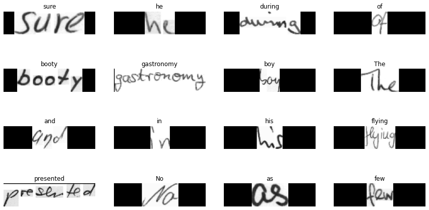
您会注意到原始图像的内容尽可能忠实地得以保留,并进行了相应的填充。
模型
我们的模型将使用 CTC 损失作为端点层。有关 CTC 损失的详细信息,请参阅 这篇博文。
class CTCLayer(keras.layers.Layer):
    def __init__(self, name=None):
        super().__init__(name=name)
        self.loss_fn = tf.keras.backend.ctc_batch_cost

    def call(self, y_true, y_pred):
        batch_len = ops.cast(ops.shape(y_true)[0], dtype="int64")
        input_length = ops.cast(ops.shape(y_pred)[1], dtype="int64")
        label_length = ops.cast(ops.shape(y_true)[1], dtype="int64")

        input_length = input_length * ops.ones(shape=(batch_len, 1), dtype="int64")
        label_length = label_length * ops.ones(shape=(batch_len, 1), dtype="int64")
        loss = self.loss_fn(y_true, y_pred, input_length, label_length)
        self.add_loss(loss)

        # At test time, just return the computed predictions.
        return y_pred


def build_model():
    # Inputs to the model
    input_img = keras.Input(shape=(image_width, image_height, 1), name="image")
    labels = keras.layers.Input(name="label", shape=(None,))

    # First conv block.
    x = keras.layers.Conv2D(
        32,
        (3, 3),
        activation="relu",
        kernel_initializer="he_normal",
        padding="same",
        name="Conv1",
    )(input_img)
    x = keras.layers.MaxPooling2D((2, 2), name="pool1")(x)

    # Second conv block.
    x = keras.layers.Conv2D(
        64,
        (3, 3),
        activation="relu",
        kernel_initializer="he_normal",
        padding="same",
        name="Conv2",
    )(x)
    x = keras.layers.MaxPooling2D((2, 2), name="pool2")(x)

    # We have used two max pool with pool size and strides 2.
    # Hence, downsampled feature maps are 4x smaller. The number of
    # filters in the last layer is 64. Reshape accordingly before
    # passing the output to the RNN part of the model.
    new_shape = ((image_width // 4), (image_height // 4) * 64)
    x = keras.layers.Reshape(target_shape=new_shape, name="reshape")(x)
    x = keras.layers.Dense(64, activation="relu", name="dense1")(x)
    x = keras.layers.Dropout(0.2)(x)

    # RNNs.
    x = keras.layers.Bidirectional(
        keras.layers.LSTM(128, return_sequences=True, dropout=0.25)
    )(x)
    x = keras.layers.Bidirectional(
        keras.layers.LSTM(64, return_sequences=True, dropout=0.25)
    )(x)

    # +2 is to account for the two special tokens introduced by the CTC loss.
    # The recommendation comes here: https://git.io/J0eXP.
    x = keras.layers.Dense(
        len(char_to_num.get_vocabulary()) + 2, activation="softmax", name="dense2"
    )(x)

    # Add CTC layer for calculating CTC loss at each step.
    output = CTCLayer(name="ctc_loss")(labels, x)

    # Define the model.
    model = keras.models.Model(
        inputs=[input_img, labels], outputs=output, name="handwriting_recognizer"
    )
    # Optimizer.
    opt = keras.optimizers.Adam()
    # Compile the model and return.
    model.compile(optimizer=opt)
    return model


# Get the model.
model = build_model()
model.summary()
Model: "handwriting_recognizer"
┏━━━━━━━━━━━━━━━━━━━━━┳━━━━━━━━━━━━━━━━━━━┳━━━━━━━━━━━━┳━━━━━━━━━━━━━━━━━━━┓
┃ Layer (type)        ┃ Output Shape      ┃    Param # ┃ Connected to      ┃
┡━━━━━━━━━━━━━━━━━━━━━╇━━━━━━━━━━━━━━━━━━━╇━━━━━━━━━━━━╇━━━━━━━━━━━━━━━━━━━┩
│ image (InputLayer)  │ (None, 128, 32,   │          0 │ -                 │
│                     │ 1)                │            │                   │
├─────────────────────┼───────────────────┼────────────┼───────────────────┤
│ Conv1 (Conv2D)      │ (None, 128, 32,   │        320 │ image[0][0]       │
│                     │ 32)               │            │                   │
├─────────────────────┼───────────────────┼────────────┼───────────────────┤
│ pool1               │ (None, 64, 16,    │          0 │ Conv1[0][0]       │
│ (MaxPooling2D)      │ 32)               │            │                   │
├─────────────────────┼───────────────────┼────────────┼───────────────────┤
│ Conv2 (Conv2D)      │ (None, 64, 16,    │     18,496 │ pool1[0][0]       │
│                     │ 64)               │            │                   │
├─────────────────────┼───────────────────┼────────────┼───────────────────┤
│ pool2               │ (None, 32, 8, 64) │          0 │ Conv2[0][0]       │
│ (MaxPooling2D)      │                   │            │                   │
├─────────────────────┼───────────────────┼────────────┼───────────────────┤
│ reshape (Reshape)   │ (None, 32, 512)   │          0 │ pool2[0][0]       │
├─────────────────────┼───────────────────┼────────────┼───────────────────┤
│ dense1 (Dense)      │ (None, 32, 64)    │     32,832 │ reshape[0][0]     │
├─────────────────────┼───────────────────┼────────────┼───────────────────┤
│ dropout (Dropout)   │ (None, 32, 64)    │          0 │ dense1[0][0]      │
├─────────────────────┼───────────────────┼────────────┼───────────────────┤
│ bidirectional       │ (None, 32, 256)   │    197,632 │ dropout[0][0]     │
│ (Bidirectional)     │                   │            │                   │
├─────────────────────┼───────────────────┼────────────┼───────────────────┤
│ bidirectional_1     │ (None, 32, 128)   │    164,352 │ bidirectional[0]… │
│ (Bidirectional)     │                   │            │                   │
├─────────────────────┼───────────────────┼────────────┼───────────────────┤
│ label (InputLayer)  │ (None, None)      │          0 │ -                 │
├─────────────────────┼───────────────────┼────────────┼───────────────────┤
│ dense2 (Dense)      │ (None, 32, 81)    │     10,449 │ bidirectional_1[… │
├─────────────────────┼───────────────────┼────────────┼───────────────────┤
│ ctc_loss (CTCLayer) │ (None, 32, 81)    │          0 │ label[0][0],      │
│                     │                   │            │ dense2[0][0]      │
└─────────────────────┴───────────────────┴────────────┴───────────────────┘
Total params: 424,081 (1.62 MB)
Trainable params: 424,081 (1.62 MB)
Non-trainable params: 0 (0.00 B)
评估指标
编辑距离是评估 OCR 模型最常用的指标。在本节中,我们将实现它并将其用作回调来监控我们的模型。
为方便起见,我们首先将验证图像及其标签分开。
validation_images = []
validation_labels = []

for batch in validation_ds:
    validation_images.append(batch["image"])
    validation_labels.append(batch["label"])
现在,我们创建一个回调来监控编辑距离。
def calculate_edit_distance(labels, predictions):
    # Get a single batch and convert its labels to sparse tensors.
    saprse_labels = ops.cast(tf.sparse.from_dense(labels), dtype=tf.int64)

    # Make predictions and convert them to sparse tensors.
    input_len = np.ones(predictions.shape[0]) * predictions.shape[1]
    predictions_decoded = keras.ops.nn.ctc_decode(
        predictions, sequence_lengths=input_len
    )[0][0][:, :max_len]
    sparse_predictions = ops.cast(
        tf.sparse.from_dense(predictions_decoded), dtype=tf.int64
    )

    # Compute individual edit distances and average them out.
    edit_distances = tf.edit_distance(
        sparse_predictions, saprse_labels, normalize=False
    )
    return tf.reduce_mean(edit_distances)


class EditDistanceCallback(keras.callbacks.Callback):
    def __init__(self, pred_model):
        super().__init__()
        self.prediction_model = pred_model

    def on_epoch_end(self, epoch, logs=None):
        edit_distances = []

        for i in range(len(validation_images)):
            labels = validation_labels[i]
            predictions = self.prediction_model.predict(validation_images[i])
            edit_distances.append(calculate_edit_distance(labels, predictions).numpy())

        print(
            f"Mean edit distance for epoch {epoch + 1}: {np.mean(edit_distances):.4f}"
        )
训练
现在我们可以开始模型训练了。
epochs = 10  # To get good results this should be at least 50.

model = build_model()
prediction_model = keras.models.Model(
    model.get_layer(name="image").output, model.get_layer(name="dense2").output
)
edit_distance_callback = EditDistanceCallback(prediction_model)

# Train the model.
history = model.fit(
    train_ds,
    validation_data=validation_ds,
    epochs=epochs,
    callbacks=[edit_distance_callback],
)
Epoch 1/10
  1357/1357 ━━━━━━━━━━━━━━━━━━━━ 216s 157ms/step - loss: 1068.7206 - val_loss: 762.4462

Epoch 2/10
  1357/1357 ━━━━━━━━━━━━━━━━━━━━ 215s 158ms/step - loss: 735.8929 - val_loss: 627.9722

Epoch 3/10
  1357/1357 ━━━━━━━━━━━━━━━━━━━━ 211s 155ms/step - loss: 624.9929 - val_loss: 540.8905

Epoch 4/10
  1357/1357 ━━━━━━━━━━━━━━━━━━━━ 208s 153ms/step - loss: 544.2097 - val_loss: 446.0919

Epoch 5/10
  1357/1357 ━━━━━━━━━━━━━━━━━━━━ 213s 157ms/step - loss: 459.0329 - val_loss: 347.1689

Epoch 6/10
  1357/1357 ━━━━━━━━━━━━━━━━━━━━ 210s 155ms/step - loss: 378.6367 - val_loss: 287.1726

Epoch 7/10
  1357/1357 ━━━━━━━━━━━━━━━━━━━━ 211s 155ms/step - loss: 325.4126 - val_loss: 250.3677

Epoch 8/10
  1357/1357 ━━━━━━━━━━━━━━━━━━━━ 209s 154ms/step - loss: 289.2796 - val_loss: 224.4595

Epoch 9/10
  1357/1357 ━━━━━━━━━━━━━━━━━━━━ 209s 154ms/step - loss: 264.0461 - val_loss: 205.5910

Epoch 10/10
  1357/1357 ━━━━━━━━━━━━━━━━━━━━ 208s 153ms/step - loss: 245.5216 - val_loss: 195.7952
推理
# A utility function to decode the output of the network.
def decode_batch_predictions(pred):
    input_len = np.ones(pred.shape[0]) * pred.shape[1]
    # Use greedy search. For complex tasks, you can use beam search.
    results = keras.ops.nn.ctc_decode(pred, sequence_lengths=input_len)[0][0][
        :, :max_len
    ]
    # Iterate over the results and get back the text.
    output_text = []
    for res in results:
        res = tf.gather(res, tf.where(tf.math.not_equal(res, -1)))
        res = (
            tf.strings.reduce_join(num_to_char(res))
            .numpy()
            .decode("utf-8")
            .replace("[UNK]", "")
        )
        output_text.append(res)
    return output_text


#  Let's check results on some test samples.
for batch in test_ds.take(1):
    batch_images = batch["image"]
    _, ax = plt.subplots(4, 4, figsize=(15, 8))

    preds = prediction_model.predict(batch_images)
    pred_texts = decode_batch_predictions(preds)

    for i in range(16):
        img = batch_images[i]
        img = tf.image.flip_left_right(img)
        img = ops.transpose(img, (1, 0, 2))
        img = (img * 255.0).numpy().clip(0, 255).astype(np.uint8)
        img = img[:, :, 0]

        title = f"Prediction: {pred_texts[i]}"
        ax[i // 4, i % 4].imshow(img, cmap="gray")
        ax[i // 4, i % 4].set_title(title)
        ax[i // 4, i % 4].axis("off")

plt.show()
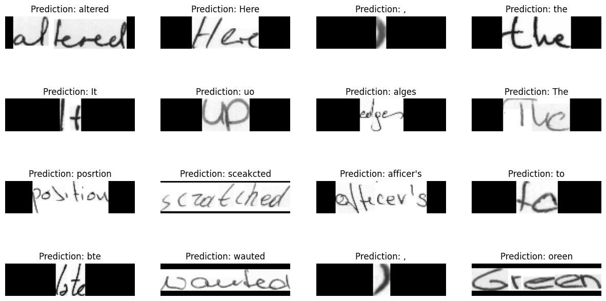
为了获得更好的结果,模型应至少训练 50 个 epoch。
最后说明
prediction_model与 TensorFlow Lite 完全兼容。如果您有兴趣,可以在移动应用程序中使用它。您可能会发现 这个 notebook 在这方面很有用。- 并非所有训练示例都完全对齐,正如本示例中所观察到的。这可能会损害模型在复杂序列上的性能。为此,我们可以利用空间变换网络(Jaderberg 等人),它可以帮助模型学习仿射变换,从而最大限度地提高其性能。