► 代码示例 / 计算机视觉 / 带有 LayerScale 的类别注意力图像 Transformer

带有 LayerScale 的类别注意力图像 Transformer

作者：Sayak Paul
创建日期 2022/09/19
最后修改日期 2022/11/21
描述： 实现一个配备类别注意力和 LayerScale 的图像 Transformer。

ⓘ 本示例使用 Keras 3

简介

在本教程中，我们将实现 Touvron 等人在《Going deeper with Image Transformers》中提出的 CaiT (Class-Attention in Image Transformers)。深度缩放，即增加模型深度以获得更好的性能和泛化能力，对于卷积神经网络来说非常成功（例如，Tan 等人，Dollár 等人）。但是，将相同的模型缩放原理应用于 Vision Transformer（Dosovitskiy 等人）并不像预期的那样有效——它们的性能随着深度缩放而迅速饱和。请注意，这里的假设是，在进行模型缩放时，始终保持底层的预训练数据集不变。

在 CaiT 的论文中，作者们研究了这种现象，并对 vanilla ViT (Vision Transformers) 架构进行了修改以缓解这个问题。

本教程的结构如下：

实现 CaiT 的各个模块
将所有模块组合起来创建 CaiT 模型
加载预训练的 CaiT 模型
获取预测结果
可视化 CaiT 的不同注意力层

假设读者已经熟悉 Vision Transformers。这里是 Keras 中 Vision Transformers 的实现：使用 Vision Transformer 进行图像分类。

导入

import os

os.environ["KERAS_BACKEND"] = "tensorflow"

import io
import typing
from urllib.request import urlopen

import matplotlib.pyplot as plt
import numpy as np
import PIL
import keras
from keras import layers
from keras import ops

LayerScale 层

我们首先实现 **LayerScale** 层，这是 CaiT 论文中提出的两种修改之一。

当增加 ViT 模型深度时，它们会遇到优化不稳定问题，并最终无法收敛。Transformer 块内的残差连接引入了信息瓶颈。当深度增加时，这个瓶颈会迅速爆炸，并偏离底层模型的优化路径。

以下方程表示残差连接在 Transformer 块内的添加位置：

其中，**SA** 代表自注意力，**FFN** 代表前馈网络，**eta** 代表 LayerNorm 运算符（Ba 等人）。

LayerScale 的正式实现如下：

其中，lambda 是可学习参数，并初始化为一个非常小的值（{0.1, 1e-5, 1e-6}）。**diag** 代表一个对角矩阵。

直观地说，LayerScale 有助于控制残差分支的贡献。LayerScale 的可学习参数被初始化为一个较小的值，以使分支充当身份函数，然后让它们在训练过程中确定交互的程度。对角矩阵此外还有一个好处，因为它是在每个通道上应用的，所以有助于控制残差输入各个维度的贡献。

LayerScale 的实际实现比听起来要简单。

class LayerScale(layers.Layer):
    """LayerScale as introduced in CaiT: https://arxiv.org/abs/2103.17239.

    Args:
        init_values (float): value to initialize the diagonal matrix of LayerScale.
        projection_dim (int): projection dimension used in LayerScale.
    """

    def __init__(self, init_values: float, projection_dim: int, **kwargs):
        super().__init__(**kwargs)
        self.gamma = self.add_weight(
            shape=(projection_dim,),
            initializer=keras.initializers.Constant(init_values),
        )

    def call(self, x, training=False):
        return x * self.gamma

随机深度层

自其引入以来（Huang 等人），随机深度已成为几乎所有现代神经网络架构中的首选组件。CaiT 也不例外。本笔记本不讨论随机深度。如果您需要回顾，请参考此资源。

class StochasticDepth(layers.Layer):
    """Stochastic Depth layer (https://arxiv.org/abs/1603.09382).

    Reference:
        https://github.com/rwightman/pytorch-image-models
    """

    def __init__(self, drop_prob: float, **kwargs):
        super().__init__(**kwargs)
        self.drop_prob = drop_prob
        self.seed_generator = keras.random.SeedGenerator(1337)

    def call(self, x, training=False):
        if training:
            keep_prob = 1 - self.drop_prob
            shape = (ops.shape(x)[0],) + (1,) * (len(x.shape) - 1)
            random_tensor = keep_prob + ops.random.uniform(
                shape, minval=0, maxval=1, seed=self.seed_generator
            )
            random_tensor = ops.floor(random_tensor)
            return (x / keep_prob) * random_tensor
        return x

类别注意力

Vanilla ViT 使用自注意力 (SA) 层来模拟图像块和**可学习的** CLS token 之间如何相互作用。CaiT 的作者建议将负责关注图像块和 CLS token 的注意力层解耦。

当对 ViTs 用于任何判别性任务（例如分类）时，我们通常会采用属于 CLS token 的表示，然后将其传递给特定于任务的头部。这与在卷积神经网络中通常使用的全局平均池化等方法形成对比。

CLS token 与其他图像块之间的交互通过自注意力层统一处理。正如 CaiT 的作者指出的那样，这种设置会产生一种纠缠效应。一方面，自注意力层负责建模图像块。另一方面，它们还负责通过 CLS token 总结建模的信息，以便其可用于学习目标。

为了帮助区分这两者，作者们建议：

在网络的后期引入 CLS token。
通过一组单独的注意力层对 CLS token 与图像块相关表示之间的交互进行建模。作者称之为**类别注意力** (CA)。

下图（摘自原始论文）描绘了这个想法：

这通过将 CLS token 嵌入视为 CA 层中的查询来实现。CLS token 嵌入和图像块嵌入被作为键和值馈送。

**注意**，“嵌入”和“表示”在这里可以互换使用。

class ClassAttention(layers.Layer):
    """Class attention as proposed in CaiT: https://arxiv.org/abs/2103.17239.

    Args:
        projection_dim (int): projection dimension for the query, key, and value
            of attention.
        num_heads (int): number of attention heads.
        dropout_rate (float): dropout rate to be used for dropout in the attention
            scores as well as the final projected outputs.
    """

    def __init__(
        self, projection_dim: int, num_heads: int, dropout_rate: float, **kwargs
    ):
        super().__init__(**kwargs)
        self.num_heads = num_heads

        head_dim = projection_dim // num_heads
        self.scale = head_dim**-0.5

        self.q = layers.Dense(projection_dim)
        self.k = layers.Dense(projection_dim)
        self.v = layers.Dense(projection_dim)
        self.attn_drop = layers.Dropout(dropout_rate)
        self.proj = layers.Dense(projection_dim)
        self.proj_drop = layers.Dropout(dropout_rate)

    def call(self, x, training=False):
        batch_size, num_patches, num_channels = (
            ops.shape(x)[0],
            ops.shape(x)[1],
            ops.shape(x)[2],
        )

        # Query projection. `cls_token` embeddings are queries.
        q = ops.expand_dims(self.q(x[:, 0]), axis=1)
        q = ops.reshape(
            q, (batch_size, 1, self.num_heads, num_channels // self.num_heads)
        )  # Shape: (batch_size, 1, num_heads, dimension_per_head)
        q = ops.transpose(q, axes=[0, 2, 1, 3])
        scale = ops.cast(self.scale, dtype=q.dtype)
        q = q * scale

        # Key projection. Patch embeddings as well the cls embedding are used as keys.
        k = self.k(x)
        k = ops.reshape(
            k, (batch_size, num_patches, self.num_heads, num_channels // self.num_heads)
        )  # Shape: (batch_size, num_tokens, num_heads, dimension_per_head)
        k = ops.transpose(k, axes=[0, 2, 3, 1])

        # Value projection. Patch embeddings as well the cls embedding are used as values.
        v = self.v(x)
        v = ops.reshape(
            v, (batch_size, num_patches, self.num_heads, num_channels // self.num_heads)
        )
        v = ops.transpose(v, axes=[0, 2, 1, 3])

        # Calculate attention scores between cls_token embedding and patch embeddings.
        attn = ops.matmul(q, k)
        attn = ops.nn.softmax(attn, axis=-1)
        attn = self.attn_drop(attn, training=training)

        x_cls = ops.matmul(attn, v)
        x_cls = ops.transpose(x_cls, axes=[0, 2, 1, 3])
        x_cls = ops.reshape(x_cls, (batch_size, 1, num_channels))
        x_cls = self.proj(x_cls)
        x_cls = self.proj_drop(x_cls, training=training)

        return x_cls, attn

Talking Head 注意力

CaiT 作者使用了 Talking Head 注意力（Shazeer 等人），而不是原始 Transformer 论文（Vaswani 等人）中使用的 vanilla 缩放点积多头注意力。他们引入了两个线性投影，分别在 softmax 操作之前和之后，以获得更好的结果。

有关 Talking Head 注意力和 vanilla 注意力机制更严谨的阐述，请参考它们各自的论文（上面已链接）。

class TalkingHeadAttention(layers.Layer):
    """Talking-head attention as proposed in CaiT: https://arxiv.org/abs/2003.02436.

    Args:
        projection_dim (int): projection dimension for the query, key, and value
            of attention.
        num_heads (int): number of attention heads.
        dropout_rate (float): dropout rate to be used for dropout in the attention
            scores as well as the final projected outputs.
    """

    def __init__(
        self, projection_dim: int, num_heads: int, dropout_rate: float, **kwargs
    ):
        super().__init__(**kwargs)

        self.num_heads = num_heads

        head_dim = projection_dim // self.num_heads

        self.scale = head_dim**-0.5

        self.qkv = layers.Dense(projection_dim * 3)
        self.attn_drop = layers.Dropout(dropout_rate)

        self.proj = layers.Dense(projection_dim)

        self.proj_l = layers.Dense(self.num_heads)
        self.proj_w = layers.Dense(self.num_heads)

        self.proj_drop = layers.Dropout(dropout_rate)

    def call(self, x, training=False):
        B, N, C = ops.shape(x)[0], ops.shape(x)[1], ops.shape(x)[2]

        # Project the inputs all at once.
        qkv = self.qkv(x)

        # Reshape the projected output so that they're segregated in terms of
        # query, key, and value projections.
        qkv = ops.reshape(qkv, (B, N, 3, self.num_heads, C // self.num_heads))

        # Transpose so that the `num_heads` becomes the leading dimensions.
        # Helps to better segregate the representation sub-spaces.
        qkv = ops.transpose(qkv, axes=[2, 0, 3, 1, 4])
        scale = ops.cast(self.scale, dtype=qkv.dtype)
        q, k, v = qkv[0] * scale, qkv[1], qkv[2]

        # Obtain the raw attention scores.
        attn = ops.matmul(q, ops.transpose(k, axes=[0, 1, 3, 2]))

        # Linear projection of the similarities between the query and key projections.
        attn = self.proj_l(ops.transpose(attn, axes=[0, 2, 3, 1]))

        # Normalize the attention scores.
        attn = ops.transpose(attn, axes=[0, 3, 1, 2])
        attn = ops.nn.softmax(attn, axis=-1)

        # Linear projection on the softmaxed scores.
        attn = self.proj_w(ops.transpose(attn, axes=[0, 2, 3, 1]))
        attn = ops.transpose(attn, axes=[0, 3, 1, 2])
        attn = self.attn_drop(attn, training=training)

        # Final set of projections as done in the vanilla attention mechanism.
        x = ops.matmul(attn, v)
        x = ops.transpose(x, axes=[0, 2, 1, 3])
        x = ops.reshape(x, (B, N, C))

        x = self.proj(x)
        x = self.proj_drop(x, training=training)

        return x, attn

前馈网络

接下来，我们实现前馈网络，它是 Transformer 块的组成部分之一。

def mlp(x, dropout_rate: float, hidden_units: typing.List[int]):
    """FFN for a Transformer block."""
    for idx, units in enumerate(hidden_units):
        x = layers.Dense(
            units,
            activation=ops.nn.gelu if idx == 0 else None,
            bias_initializer=keras.initializers.RandomNormal(stddev=1e-6),
        )(x)
        x = layers.Dropout(dropout_rate)(x)
    return x

其他模块

在接下来的两个单元格中，我们将剩余的模块实现为独立函数：

LayerScaleBlockClassAttention() 返回一个 keras.Model。它是一个配备类别注意力、LayerScale 和随机深度的 Transformer 块。它作用于 CLS 嵌入和图像块嵌入。
LayerScaleBlock() 返回一个 keras.model。它也是一个 Transformer 块，仅作用于图像块的嵌入。它配备了 LayerScale 和随机深度。

def LayerScaleBlockClassAttention(
    projection_dim: int,
    num_heads: int,
    layer_norm_eps: float,
    init_values: float,
    mlp_units: typing.List[int],
    dropout_rate: float,
    sd_prob: float,
    name: str,
):
    """Pre-norm transformer block meant to be applied to the embeddings of the
    cls token and the embeddings of image patches.

    Includes LayerScale and Stochastic Depth.

    Args:
        projection_dim (int): projection dimension to be used in the
            Transformer blocks and patch projection layer.
        num_heads (int): number of attention heads.
        layer_norm_eps (float): epsilon to be used for Layer Normalization.
        init_values (float): initial value for the diagonal matrix used in LayerScale.
        mlp_units (List[int]): dimensions of the feed-forward network used in
            the Transformer blocks.
        dropout_rate (float): dropout rate to be used for dropout in the attention
            scores as well as the final projected outputs.
        sd_prob (float): stochastic depth rate.
        name (str): a name identifier for the block.

    Returns:
        A keras.Model instance.
    """
    x = keras.Input((None, projection_dim))
    x_cls = keras.Input((None, projection_dim))
    inputs = keras.layers.Concatenate(axis=1)([x_cls, x])

    # Class attention (CA).
    x1 = layers.LayerNormalization(epsilon=layer_norm_eps)(inputs)
    attn_output, attn_scores = ClassAttention(projection_dim, num_heads, dropout_rate)(
        x1
    )
    attn_output = (
        LayerScale(init_values, projection_dim)(attn_output)
        if init_values
        else attn_output
    )
    attn_output = StochasticDepth(sd_prob)(attn_output) if sd_prob else attn_output
    x2 = keras.layers.Add()([x_cls, attn_output])

    # FFN.
    x3 = layers.LayerNormalization(epsilon=layer_norm_eps)(x2)
    x4 = mlp(x3, hidden_units=mlp_units, dropout_rate=dropout_rate)
    x4 = LayerScale(init_values, projection_dim)(x4) if init_values else x4
    x4 = StochasticDepth(sd_prob)(x4) if sd_prob else x4
    outputs = keras.layers.Add()([x2, x4])

    return keras.Model([x, x_cls], [outputs, attn_scores], name=name)


def LayerScaleBlock(
    projection_dim: int,
    num_heads: int,
    layer_norm_eps: float,
    init_values: float,
    mlp_units: typing.List[int],
    dropout_rate: float,
    sd_prob: float,
    name: str,
):
    """Pre-norm transformer block meant to be applied to the embeddings of the
    image patches.

    Includes LayerScale and Stochastic Depth.

        Args:
            projection_dim (int): projection dimension to be used in the
                Transformer blocks and patch projection layer.
            num_heads (int): number of attention heads.
            layer_norm_eps (float): epsilon to be used for Layer Normalization.
            init_values (float): initial value for the diagonal matrix used in LayerScale.
            mlp_units (List[int]): dimensions of the feed-forward network used in
                the Transformer blocks.
            dropout_rate (float): dropout rate to be used for dropout in the attention
                scores as well as the final projected outputs.
            sd_prob (float): stochastic depth rate.
            name (str): a name identifier for the block.

    Returns:
        A keras.Model instance.
    """
    encoded_patches = keras.Input((None, projection_dim))

    # Self-attention.
    x1 = layers.LayerNormalization(epsilon=layer_norm_eps)(encoded_patches)
    attn_output, attn_scores = TalkingHeadAttention(
        projection_dim, num_heads, dropout_rate
    )(x1)
    attn_output = (
        LayerScale(init_values, projection_dim)(attn_output)
        if init_values
        else attn_output
    )
    attn_output = StochasticDepth(sd_prob)(attn_output) if sd_prob else attn_output
    x2 = layers.Add()([encoded_patches, attn_output])

    # FFN.
    x3 = layers.LayerNormalization(epsilon=layer_norm_eps)(x2)
    x4 = mlp(x3, hidden_units=mlp_units, dropout_rate=dropout_rate)
    x4 = LayerScale(init_values, projection_dim)(x4) if init_values else x4
    x4 = StochasticDepth(sd_prob)(x4) if sd_prob else x4
    outputs = layers.Add()([x2, x4])

    return keras.Model(encoded_patches, [outputs, attn_scores], name=name)

有了所有这些模块，我们就可以将它们组合成最终的 CaiT 模型了。

将各个部分组合在一起：CaiT 模型

class CaiT(keras.Model):
    """CaiT model.

    Args:
        projection_dim (int): projection dimension to be used in the
            Transformer blocks and patch projection layer.
        patch_size (int): patch size of the input images.
        num_patches (int): number of patches after extracting the image patches.
        init_values (float): initial value for the diagonal matrix used in LayerScale.
        mlp_units: (List[int]): dimensions of the feed-forward network used in
            the Transformer blocks.
        sa_ffn_layers (int): number of self-attention Transformer blocks.
        ca_ffn_layers (int): number of class-attention Transformer blocks.
        num_heads (int): number of attention heads.
        layer_norm_eps (float): epsilon to be used for Layer Normalization.
        dropout_rate (float): dropout rate to be used for dropout in the attention
            scores as well as the final projected outputs.
        sd_prob (float): stochastic depth rate.
        global_pool (str): denotes how to pool the representations coming out of
            the final Transformer block.
        pre_logits (bool): if set to True then don't add a classification head.
        num_classes (int): number of classes to construct the final classification
            layer with.
    """

    def __init__(
        self,
        projection_dim: int,
        patch_size: int,
        num_patches: int,
        init_values: float,
        mlp_units: typing.List[int],
        sa_ffn_layers: int,
        ca_ffn_layers: int,
        num_heads: int,
        layer_norm_eps: float,
        dropout_rate: float,
        sd_prob: float,
        global_pool: str,
        pre_logits: bool,
        num_classes: int,
        **kwargs,
    ):
        if global_pool not in ["token", "avg"]:
            raise ValueError(
                'Invalid value received for `global_pool`, should be either `"token"` or `"avg"`.'
            )

        super().__init__(**kwargs)

        # Responsible for patchifying the input images and the linearly projecting them.
        self.projection = keras.Sequential(
            [
                layers.Conv2D(
                    filters=projection_dim,
                    kernel_size=(patch_size, patch_size),
                    strides=(patch_size, patch_size),
                    padding="VALID",
                    name="conv_projection",
                    kernel_initializer="lecun_normal",
                ),
                layers.Reshape(
                    target_shape=(-1, projection_dim),
                    name="flatten_projection",
                ),
            ],
            name="projection",
        )

        # CLS token and the positional embeddings.
        self.cls_token = self.add_weight(
            shape=(1, 1, projection_dim), initializer="zeros"
        )
        self.pos_embed = self.add_weight(
            shape=(1, num_patches, projection_dim), initializer="zeros"
        )

        # Projection dropout.
        self.pos_drop = layers.Dropout(dropout_rate, name="projection_dropout")

        # Stochastic depth schedule.
        dpr = [sd_prob for _ in range(sa_ffn_layers)]

        # Self-attention (SA) Transformer blocks operating only on the image patch
        # embeddings.
        self.blocks = [
            LayerScaleBlock(
                projection_dim=projection_dim,
                num_heads=num_heads,
                layer_norm_eps=layer_norm_eps,
                init_values=init_values,
                mlp_units=mlp_units,
                dropout_rate=dropout_rate,
                sd_prob=dpr[i],
                name=f"sa_ffn_block_{i}",
            )
            for i in range(sa_ffn_layers)
        ]

        # Class Attention (CA) Transformer blocks operating on the CLS token and image patch
        # embeddings.
        self.blocks_token_only = [
            LayerScaleBlockClassAttention(
                projection_dim=projection_dim,
                num_heads=num_heads,
                layer_norm_eps=layer_norm_eps,
                init_values=init_values,
                mlp_units=mlp_units,
                dropout_rate=dropout_rate,
                name=f"ca_ffn_block_{i}",
                sd_prob=0.0,  # No Stochastic Depth in the class attention layers.
            )
            for i in range(ca_ffn_layers)
        ]

        # Pre-classification layer normalization.
        self.norm = layers.LayerNormalization(epsilon=layer_norm_eps, name="head_norm")

        # Representation pooling for classification head.
        self.global_pool = global_pool

        # Classification head.
        self.pre_logits = pre_logits
        self.num_classes = num_classes
        if not pre_logits:
            self.head = layers.Dense(num_classes, name="classification_head")

    def call(self, x, training=False):
        # Notice how CLS token is not added here.
        x = self.projection(x)
        x = x + self.pos_embed
        x = self.pos_drop(x)

        # SA+FFN layers.
        sa_ffn_attn = {}
        for blk in self.blocks:
            x, attn_scores = blk(x)
            sa_ffn_attn[f"{blk.name}_att"] = attn_scores

        # CA+FFN layers.
        ca_ffn_attn = {}
        cls_tokens = ops.tile(self.cls_token, (ops.shape(x)[0], 1, 1))
        for blk in self.blocks_token_only:
            cls_tokens, attn_scores = blk([x, cls_tokens])
            ca_ffn_attn[f"{blk.name}_att"] = attn_scores

        x = ops.concatenate([cls_tokens, x], axis=1)
        x = self.norm(x)

        # Always return the attention scores from the SA+FFN and CA+FFN layers
        # for convenience.
        if self.global_pool:
            x = (
                ops.reduce_mean(x[:, 1:], axis=1)
                if self.global_pool == "avg"
                else x[:, 0]
            )
        return (
            (x, sa_ffn_attn, ca_ffn_attn)
            if self.pre_logits
            else (self.head(x), sa_ffn_attn, ca_ffn_attn)
        )

将 SA 和 CA 层这样分开有助于模型更具体地关注底层目标：

图像块之间的模型依赖关系
在 CLS token 中总结图像块信息，以便可以用于当前任务

既然我们已经定义了 CaiT 模型，现在是时候进行测试了。我们将从定义一个模型配置开始，该配置将传递给我们的 CaiT 类进行初始化。

定义模型配置

def get_config(
    image_size: int = 224,
    patch_size: int = 16,
    projection_dim: int = 192,
    sa_ffn_layers: int = 24,
    ca_ffn_layers: int = 2,
    num_heads: int = 4,
    mlp_ratio: int = 4,
    layer_norm_eps=1e-6,
    init_values: float = 1e-5,
    dropout_rate: float = 0.0,
    sd_prob: float = 0.0,
    global_pool: str = "token",
    pre_logits: bool = False,
    num_classes: int = 1000,
) -> typing.Dict:
    """Default configuration for CaiT models (cait_xxs24_224).

    Reference:
        https://github.com/rwightman/pytorch-image-models/blob/master/timm/models/cait.py
    """
    config = {}

    # Patchification and projection.
    config["patch_size"] = patch_size
    config["num_patches"] = (image_size // patch_size) ** 2

    # LayerScale.
    config["init_values"] = init_values

    # Dropout and Stochastic Depth.
    config["dropout_rate"] = dropout_rate
    config["sd_prob"] = sd_prob

    # Shared across different blocks and layers.
    config["layer_norm_eps"] = layer_norm_eps
    config["projection_dim"] = projection_dim
    config["mlp_units"] = [
        projection_dim * mlp_ratio,
        projection_dim,
    ]

    # Attention layers.
    config["num_heads"] = num_heads
    config["sa_ffn_layers"] = sa_ffn_layers
    config["ca_ffn_layers"] = ca_ffn_layers

    # Representation pooling and task specific parameters.
    config["global_pool"] = global_pool
    config["pre_logits"] = pre_logits
    config["num_classes"] = num_classes

    return config

如果您已经了解 ViT 架构，那么大多数配置变量对您来说应该都很熟悉。重点关注 sa_ffn_layers 和 ca_ffn_layers，它们控制 SA-Transformer 块和 CA-Transformer 块的数量。您可以轻松修改此 get_config() 方法来为自己的数据集实例化 CaiT 模型。

模型实例化

image_size = 224
num_channels = 3
batch_size = 2

config = get_config()
cait_xxs24_224 = CaiT(**config)

dummy_inputs = ops.ones((batch_size, image_size, image_size, num_channels))
_ = cait_xxs24_224(dummy_inputs)

我们可以成功地对模型进行推理。但是实现是否正确呢？有许多方法可以验证这一点：

在 ImageNet-1k 验证集上获得模型的性能（假设它已填充了预训练参数）（因为预训练数据集是 ImageNet-1k）。
在不同的数据集上微调模型。

为了验证这一点，我们将加载另一个相同模型的实例，该实例已填充了预训练参数。有关更多详细信息，请参考这个仓库（由本笔记本的作者开发）。此外，该存储库还提供了用于验证模型在ImageNet-1k 验证集上性能以及微调的代码。

加载预训练模型

model_gcs_path = "gs://kaggle-tfhub-models-uncompressed/tfhub-modules/sayakpaul/cait_xxs24_224/1/uncompressed"
pretrained_model = keras.Sequential(
    [keras.layers.TFSMLayer(model_gcs_path, call_endpoint="serving_default")]
)

推理工具

在接下来的几个单元格中，我们将开发预处理工具，以运行预训练模型的推理。

# The preprocessing transformations include center cropping, and normalizing
# the pixel values with the ImageNet-1k training stats (mean and standard deviation).
crop_layer = keras.layers.CenterCrop(image_size, image_size)
norm_layer = keras.layers.Normalization(
    mean=[0.485 * 255, 0.456 * 255, 0.406 * 255],
    variance=[(0.229 * 255) ** 2, (0.224 * 255) ** 2, (0.225 * 255) ** 2],
)


def preprocess_image(image, size=image_size):
    image = np.array(image)
    image_resized = ops.expand_dims(image, 0)
    resize_size = int((256 / image_size) * size)
    image_resized = ops.image.resize(
        image_resized, (resize_size, resize_size), interpolation="bicubic"
    )
    image_resized = crop_layer(image_resized)
    return norm_layer(image_resized).numpy()


def load_image_from_url(url):
    image_bytes = io.BytesIO(urlopen(url).read())
    image = PIL.Image.open(image_bytes)
    preprocessed_image = preprocess_image(image)
    return image, preprocessed_image

现在，我们检索 ImageNet-1k 标签并加载它们，因为我们加载的模型是在 ImageNet-1k 数据集上预训练的。

# ImageNet-1k class labels.
imagenet_labels = (
    "https://storage.googleapis.com/bit_models/ilsvrc2012_wordnet_lemmas.txt"
)
label_path = keras.utils.get_file(origin=imagenet_labels)

with open(label_path, "r") as f:
    lines = f.readlines()
imagenet_labels = [line.rstrip() for line in lines]

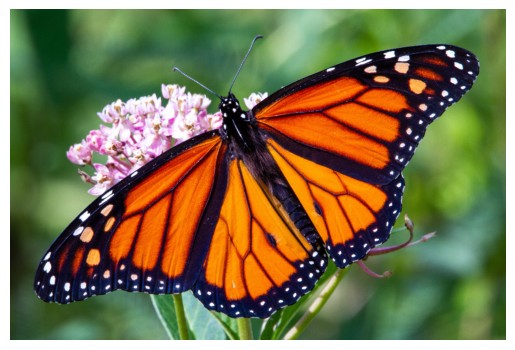
加载图像

img_url = "https://i.imgur.com/ErgfLTn.jpg"
image, preprocessed_image = load_image_from_url(img_url)

# https://unsplash.com/photos/Ho93gVTRWW8
plt.imshow(image)
plt.axis("off")
plt.show()

png

获取预测

outputs = pretrained_model.predict(preprocessed_image)
logits = outputs["output_1"]
ca_ffn_block_0_att = outputs["output_3_ca_ffn_block_0_att"]
ca_ffn_block_1_att = outputs["output_3_ca_ffn_block_1_att"]

predicted_label = imagenet_labels[int(np.argmax(logits))]
print(predicted_label)

 1/1 ━━━━━━━━━━━━━━━━━━━━ 30s 30s/step
monarch, monarch_butterfly, milkweed_butterfly, Danaus_plexippus

WARNING: All log messages before absl::InitializeLog() is called are written to STDERR
I0000 00:00:1700601113.319904  361514 device_compiler.h:187] Compiled cluster using XLA!  This line is logged at most once for the lifetime of the process.

既然我们已经获得了预测（它们似乎符合预期），我们可以进一步扩展我们的研究。遵循 CaiT 作者的思路，我们可以检查来自注意力层的注意力分数。这有助于我们更深入地了解 CaiT 论文中引入的修改。

可视化注意力层

我们首先检查类别注意力层返回的注意力权重的形状。

# (batch_size, nb_attention_heads, num_cls_token, seq_length)
print("Shape of the attention scores from a class attention block:")
print(ca_ffn_block_0_att.shape)

Shape of the attention scores from a class attention block:
(1, 4, 1, 197)

该形状表示我们获得了每个单独注意力头的注意力权重。它们量化了 CLS token 如何与自身以及其余图像块相关的信息。

接下来，我们编写一个工具来：

可视化类别注意力层中各个注意力头正在关注的内容。这有助于我们了解 CaiT 模型是如何引入**空间-类别关系**的。
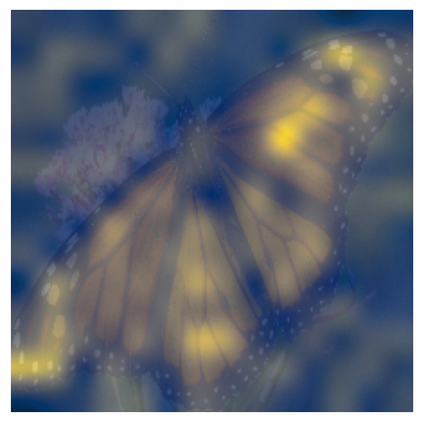
从第一个类别注意力层获取一个显著图，以帮助理解 CA 层如何从图像中的感兴趣区域聚合信息。

此工具参考了原始CaiT 论文的图 6 和图 7。这也是这个笔记本（由本教程作者开发）的一部分。

# Reference:
# https://github.com/facebookresearch/dino/blob/main/visualize_attention.py

patch_size = 16


def get_cls_attention_map(
    attention_scores,
    return_saliency=False,
) -> np.ndarray:
    """
    Returns attention scores from a particular attention block.

    Args:
        attention_scores: the attention scores from the attention block to
            visualize.
        return_saliency: a boolean flag if set to True also returns the salient
            representations of the attention block.
    """
    w_featmap = preprocessed_image.shape[2] // patch_size
    h_featmap = preprocessed_image.shape[1] // patch_size

    nh = attention_scores.shape[1]  # Number of attention heads.

    # Taking the representations from CLS token.
    attentions = attention_scores[0, :, 0, 1:].reshape(nh, -1)

    # Reshape the attention scores to resemble mini patches.
    attentions = attentions.reshape(nh, w_featmap, h_featmap)

    if not return_saliency:
        attentions = attentions.transpose((1, 2, 0))

    else:
        attentions = np.mean(attentions, axis=0)
        attentions = (attentions - attentions.min()) / (
            attentions.max() - attentions.min()
        )
        attentions = np.expand_dims(attentions, -1)

    # Resize the attention patches to 224x224 (224: 14x16)
    attentions = ops.image.resize(
        attentions,
        size=(h_featmap * patch_size, w_featmap * patch_size),
        interpolation="bicubic",
    )

    return attentions

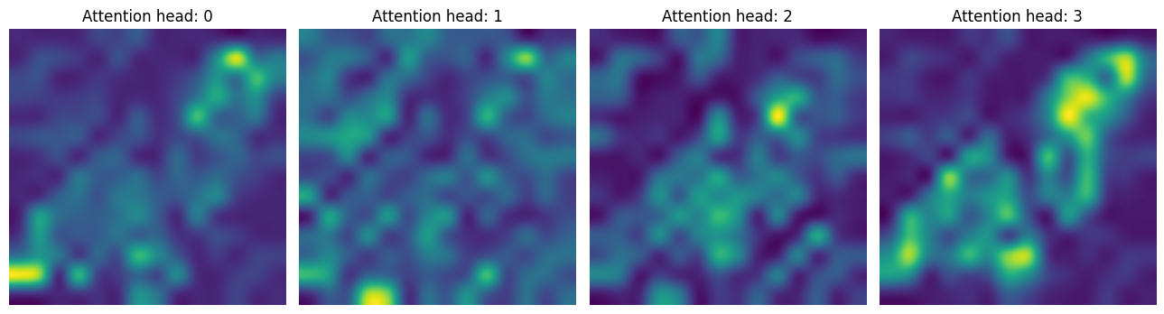
在第一个 CA 层中，我们注意到模型仅关注感兴趣的区域。

attentions_ca_block_0 = get_cls_attention_map(ca_ffn_block_0_att)


fig, axes = plt.subplots(nrows=1, ncols=4, figsize=(13, 13))
img_count = 0

for i in range(attentions_ca_block_0.shape[-1]):
    if img_count < attentions_ca_block_0.shape[-1]:
        axes[i].imshow(attentions_ca_block_0[:, :, img_count])
        axes[i].title.set_text(f"Attention head: {img_count}")
        axes[i].axis("off")
        img_count += 1

fig.tight_layout()
plt.show()

png

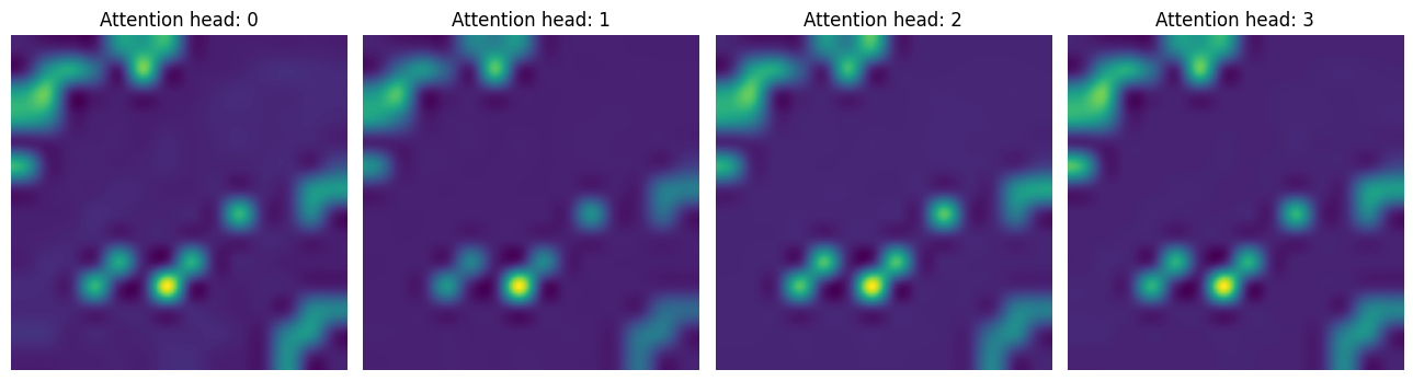
而在第二个 CA 层中，模型则试图更多地关注包含判别性信号的上下文。

attentions_ca_block_1 = get_cls_attention_map(ca_ffn_block_1_att)


fig, axes = plt.subplots(nrows=1, ncols=4, figsize=(13, 13))
img_count = 0

for i in range(attentions_ca_block_1.shape[-1]):
    if img_count < attentions_ca_block_1.shape[-1]:
        axes[i].imshow(attentions_ca_block_1[:, :, img_count])
        axes[i].title.set_text(f"Attention head: {img_count}")
        axes[i].axis("off")
        img_count += 1

fig.tight_layout()
plt.show()

png

最后，我们获取给定图像的显著图。

saliency_attention = get_cls_attention_map(ca_ffn_block_0_att, return_saliency=True)

image = np.array(image)
image_resized = ops.expand_dims(image, 0)
resize_size = int((256 / 224) * image_size)
image_resized = ops.image.resize(
    image_resized, (resize_size, resize_size), interpolation="bicubic"
)
image_resized = crop_layer(image_resized)

plt.imshow(image_resized.numpy().squeeze().astype("int32"))
plt.imshow(saliency_attention.numpy().squeeze(), cmap="cividis", alpha=0.9)
plt.axis("off")

plt.show()