► 开发者指南 / 使用内置方法进行训练与评估

使用内置方法进行训练与评估

作者: fchollet
创建日期 2019/03/01
最后修改日期 2023/06/25
描述: 关于使用 fit() 和 evaluate() 进行训练与评估的完整指南。

设置

# We import torch & TF so as to use torch Dataloaders & tf.data.Datasets.
import torch
import tensorflow as tf

import os
import numpy as np
import keras
from keras import layers
from keras import ops

介绍

本指南涵盖了在使用内置 API（如 Model.fit()、Model.evaluate() 和 Model.predict()）进行训练与验证时，模型的训练、评估和预测（推理）。

如果你对利用 fit() 同时指定自己的训练步骤函数感兴趣，请参阅关于如何自定义 fit() 行为的指南。

如果你对从头开始编写自己的训练与评估循环感兴趣，请参阅关于编写训练循环的指南。

通常来说，无论你使用内置循环还是自己编写循环，模型训练与评估在所有类型的 Keras 模型中工作方式都严格一致——无论是 Sequential 模型、使用函数式 API 构建的模型，还是通过模型子类化从头编写的模型。

API 概览：第一个端到端示例

将数据传递给模型的内置训练循环时，应使用以下任一方式：

NumPy 数组（如果数据量小且能放入内存）
keras.utils.PyDataset 的子类
tf.data.Dataset 对象
PyTorch DataLoader 实例

在接下来的几段中，我们将使用 MNIST 数据集作为 NumPy 数组，以演示如何使用优化器、损失函数和指标。之后，我们将详细探讨其他每种选项。

让我们考虑以下模型（这里我们使用函数式 API 构建，但它也可以是 Sequential 模型或子类化模型）

inputs = keras.Input(shape=(784,), name="digits")
x = layers.Dense(64, activation="relu", name="dense_1")(inputs)
x = layers.Dense(64, activation="relu", name="dense_2")(x)
outputs = layers.Dense(10, activation="softmax", name="predictions")(x)

model = keras.Model(inputs=inputs, outputs=outputs)

典型的端到端工作流程如下所示，包括：

训练
在从原始训练数据生成的保留集上进行验证
在测试数据上进行评估

本例我们将使用 MNIST 数据。

(x_train, y_train), (x_test, y_test) = keras.datasets.mnist.load_data()

# Preprocess the data (these are NumPy arrays)
x_train = x_train.reshape(60000, 784).astype("float32") / 255
x_test = x_test.reshape(10000, 784).astype("float32") / 255

y_train = y_train.astype("float32")
y_test = y_test.astype("float32")

# Reserve 10,000 samples for validation
x_val = x_train[-10000:]
y_val = y_train[-10000:]
x_train = x_train[:-10000]
y_train = y_train[:-10000]

我们指定训练配置（优化器、损失函数、指标）

model.compile(
    optimizer=keras.optimizers.RMSprop(),  # Optimizer
    # Loss function to minimize
    loss=keras.losses.SparseCategoricalCrossentropy(),
    # List of metrics to monitor
    metrics=[keras.metrics.SparseCategoricalAccuracy()],
)

我们调用 fit()，它将通过将数据切片成大小为 batch_size 的“批次”，并在给定数量的 epochs 中重复遍历整个数据集来训练模型。

print("Fit model on training data")
history = model.fit(
    x_train,
    y_train,
    batch_size=64,
    epochs=2,
    # We pass some validation for
    # monitoring validation loss and metrics
    # at the end of each epoch
    validation_data=(x_val, y_val),
)

Fit model on training data
Epoch 1/2
 782/782 ━━━━━━━━━━━━━━━━━━━━ 1s 955us/step - loss: 0.5740 - sparse_categorical_accuracy: 0.8368 - val_loss: 0.2040 - val_sparse_categorical_accuracy: 0.9420
Epoch 2/2
 782/782 ━━━━━━━━━━━━━━━━━━━━ 0s 390us/step - loss: 0.1745 - sparse_categorical_accuracy: 0.9492 - val_loss: 0.1415 - val_sparse_categorical_accuracy: 0.9581

返回的 history 对象包含训练期间损失值和指标值的记录

print(history.history)

{'loss': [0.34448376297950745, 0.16419583559036255], 'sparse_categorical_accuracy': [0.9008600115776062, 0.9509199857711792], 'val_loss': [0.20404714345932007, 0.14145156741142273], 'val_sparse_categorical_accuracy': [0.9419999718666077, 0.9581000208854675]}

我们通过 evaluate() 在测试数据上评估模型

# Evaluate the model on the test data using `evaluate`
print("Evaluate on test data")
results = model.evaluate(x_test, y_test, batch_size=128)
print("test loss, test acc:", results)

# Generate predictions (probabilities -- the output of the last layer)
# on new data using `predict`
print("Generate predictions for 3 samples")
predictions = model.predict(x_test[:3])
print("predictions shape:", predictions.shape)

Evaluate on test data
 79/79 ━━━━━━━━━━━━━━━━━━━━ 0s 271us/step - loss: 0.1670 - sparse_categorical_accuracy: 0.9489
test loss, test acc: [0.1484374850988388, 0.9550999999046326]
Generate predictions for 3 samples
 1/1 ━━━━━━━━━━━━━━━━━━━━ 0s 33ms/step
predictions shape: (3, 10)

现在，让我们详细回顾一下这个工作流程的每个部分。

`compile()` 方法：指定损失函数、指标和优化器

要使用 fit() 训练模型，需要指定一个损失函数、一个优化器，以及可选地指定一些要监控的指标。

将它们作为参数传递给模型的 compile() 方法

model.compile(
    optimizer=keras.optimizers.RMSprop(learning_rate=1e-3),
    loss=keras.losses.SparseCategoricalCrossentropy(),
    metrics=[keras.metrics.SparseCategoricalAccuracy()],
)

metrics 参数应该是一个列表——你的模型可以包含任意数量的指标。

如果你的模型有多个输出，可以为每个输出指定不同的损失函数和指标，并且可以调整每个输出对模型总损失的贡献。在**将数据传递给多输入、多输出模型**部分，你将找到更多关于此的详细信息。

请注意，如果你对默认设置满意，在许多情况下，优化器、损失函数和指标可以通过字符串标识符指定，作为一种快捷方式。

model.compile(
    optimizer="rmsprop",
    loss="sparse_categorical_crossentropy",
    metrics=["sparse_categorical_accuracy"],
)

为了将来重用，我们将模型定义和编译步骤放在函数中；在本指南的不同示例中，我们将多次调用它们。

def get_uncompiled_model():
    inputs = keras.Input(shape=(784,), name="digits")
    x = layers.Dense(64, activation="relu", name="dense_1")(inputs)
    x = layers.Dense(64, activation="relu", name="dense_2")(x)
    outputs = layers.Dense(10, activation="softmax", name="predictions")(x)
    model = keras.Model(inputs=inputs, outputs=outputs)
    return model


def get_compiled_model():
    model = get_uncompiled_model()
    model.compile(
        optimizer="rmsprop",
        loss="sparse_categorical_crossentropy",
        metrics=["sparse_categorical_accuracy"],
    )
    return model

许多内置的优化器、损失函数和指标可用

通常情况下，你无需从头开始创建自己的损失函数、指标或优化器，因为你所需的功能很可能已是 Keras API 的一部分。

优化器

SGD()（带或不带动量）
RMSprop()
Adam()
等。

损失函数

MeanSquaredError()
KLDivergence()
CosineSimilarity()
等。

指标

AUC()
Precision()
Recall()
等。

自定义损失函数

如果你需要创建自定义损失函数，Keras 提供了三种方法。

第一种方法是创建一个接受输入 y_true 和 y_pred 的函数。以下示例展示了一个计算真实数据与预测值之间均方误差的损失函数。

def custom_mean_squared_error(y_true, y_pred):
    return ops.mean(ops.square(y_true - y_pred), axis=-1)


model = get_uncompiled_model()
model.compile(optimizer=keras.optimizers.Adam(), loss=custom_mean_squared_error)

# We need to one-hot encode the labels to use MSE
y_train_one_hot = ops.one_hot(y_train, num_classes=10)
model.fit(x_train, y_train_one_hot, batch_size=64, epochs=1)

 782/782 ━━━━━━━━━━━━━━━━━━━━ 1s 525us/step - loss: 0.0277

<keras.src.callbacks.history.History at 0x2e5dde350>

如果你需要一个除了 y_true 和 y_pred 外还接受其他参数的损失函数，可以子类化 keras.losses.Loss 类并实现以下两个方法。

__init__(self)：接受在调用损失函数时传递的参数。
call(self, y_true, y_pred)：使用目标值 (y_true) 和模型预测值 (y_pred) 计算模型的损失。

假设你想使用均方误差，但添加一个惩罚项，以抑制远离 0.5 的预测值（我们假定分类目标是 one-hot 编码且取值在 0 和 1 之间）。这会促使模型不过于自信，可能有助于减少过拟合（只有尝试后才知道是否有效！）。

方法如下：

class CustomMSE(keras.losses.Loss):
    def __init__(self, regularization_factor=0.1, name="custom_mse"):
        super().__init__(name=name)
        self.regularization_factor = regularization_factor

    def call(self, y_true, y_pred):
        mse = ops.mean(ops.square(y_true - y_pred), axis=-1)
        reg = ops.mean(ops.square(0.5 - y_pred), axis=-1)
        return mse + reg * self.regularization_factor


model = get_uncompiled_model()
model.compile(optimizer=keras.optimizers.Adam(), loss=CustomMSE())

y_train_one_hot = ops.one_hot(y_train, num_classes=10)
model.fit(x_train, y_train_one_hot, batch_size=64, epochs=1)

 782/782 ━━━━━━━━━━━━━━━━━━━━ 1s 532us/step - loss: 0.0492

<keras.src.callbacks.history.History at 0x2e5d0d360>

自定义指标

如果你需要一个不在 API 中的指标，可以通过子类化 keras.metrics.Metric 类轻松创建自定义指标。你需要实现 4 个方法。

__init__(self)，用于为你的指标创建状态变量。
update_state(self, y_true, y_pred, sample_weight=None)，使用目标值 y_true 和模型预测值 y_pred 更新状态变量。
result(self)，使用状态变量计算最终结果。
reset_state(self)，重新初始化指标的状态。

状态更新和结果计算是分开的（分别在 update_state() 和 result() 中），因为在某些情况下，结果计算可能非常耗时，只会在周期性进行。

下面是一个简单的示例，展示如何实现一个 CategoricalTruePositives 指标，它统计有多少样本被正确分类到给定类别。

class CategoricalTruePositives(keras.metrics.Metric):
    def __init__(self, name="categorical_true_positives", **kwargs):
        super().__init__(name=name, **kwargs)
        self.true_positives = self.add_variable(
            shape=(), name="ctp", initializer="zeros"
        )

    def update_state(self, y_true, y_pred, sample_weight=None):
        y_pred = ops.reshape(ops.argmax(y_pred, axis=1), (-1, 1))
        values = ops.cast(y_true, "int32") == ops.cast(y_pred, "int32")
        values = ops.cast(values, "float32")
        if sample_weight is not None:
            sample_weight = ops.cast(sample_weight, "float32")
            values = ops.multiply(values, sample_weight)
        self.true_positives.assign_add(ops.sum(values))

    def result(self):
        return self.true_positives.value

    def reset_state(self):
        # The state of the metric will be reset at the start of each epoch.
        self.true_positives.assign(0.0)


model = get_uncompiled_model()
model.compile(
    optimizer=keras.optimizers.RMSprop(learning_rate=1e-3),
    loss=keras.losses.SparseCategoricalCrossentropy(),
    metrics=[CategoricalTruePositives()],
)
model.fit(x_train, y_train, batch_size=64, epochs=3)

Epoch 1/3
 782/782 ━━━━━━━━━━━━━━━━━━━━ 1s 568us/step - categorical_true_positives: 180967.9219 - loss: 0.5876
Epoch 2/3
 782/782 ━━━━━━━━━━━━━━━━━━━━ 0s 377us/step - categorical_true_positives: 182141.9375 - loss: 0.1733
Epoch 3/3
 782/782 ━━━━━━━━━━━━━━━━━━━━ 0s 377us/step - categorical_true_positives: 182303.5312 - loss: 0.1180

<keras.src.callbacks.history.History at 0x2e5f02d10>

处理不符合标准签名的损失函数和指标

绝大多数损失函数和指标都可以从 y_true 和 y_pred 计算得出，其中 y_pred 是模型的输出——但并非全部。例如，正则化损失可能只需要某层的激活（这种情况下没有目标值），并且该激活可能不是模型输出。

在这种情况下，你可以从自定义层的 call 方法内部调用 self.add_loss(loss_value)。以这种方式添加的损失会在训练期间被添加到“主”损失（传递给 compile() 的损失）中。这是一个添加活动正则化的简单示例（请注意，活动正则化已内置于所有 Keras 层中——此层仅用于提供具体示例）。

class ActivityRegularizationLayer(layers.Layer):
    def call(self, inputs):
        self.add_loss(ops.sum(inputs) * 0.1)
        return inputs  # Pass-through layer.


inputs = keras.Input(shape=(784,), name="digits")
x = layers.Dense(64, activation="relu", name="dense_1")(inputs)

# Insert activity regularization as a layer
x = ActivityRegularizationLayer()(x)

x = layers.Dense(64, activation="relu", name="dense_2")(x)
outputs = layers.Dense(10, name="predictions")(x)

model = keras.Model(inputs=inputs, outputs=outputs)
model.compile(
    optimizer=keras.optimizers.RMSprop(learning_rate=1e-3),
    loss=keras.losses.SparseCategoricalCrossentropy(from_logits=True),
)

# The displayed loss will be much higher than before
# due to the regularization component.
model.fit(x_train, y_train, batch_size=64, epochs=1)

 782/782 ━━━━━━━━━━━━━━━━━━━━ 1s 505us/step - loss: 3.4083

<keras.src.callbacks.history.History at 0x2e60226b0>

注意，当你通过 add_loss() 传递损失时，可以在调用 compile() 时不指定损失函数，因为模型已经有了要最小化的损失。

考虑以下 LogisticEndpoint 层：它接受目标值和 logits 作为输入，并通过 add_loss() 跟踪交叉熵损失。

class LogisticEndpoint(keras.layers.Layer):
    def __init__(self, name=None):
        super().__init__(name=name)
        self.loss_fn = keras.losses.BinaryCrossentropy(from_logits=True)

    def call(self, targets, logits, sample_weights=None):
        # Compute the training-time loss value and add it
        # to the layer using `self.add_loss()`.
        loss = self.loss_fn(targets, logits, sample_weights)
        self.add_loss(loss)

        # Return the inference-time prediction tensor (for `.predict()`).
        return ops.softmax(logits)

你可以在一个具有两个输入（输入数据和目标值）的模型中使用它，该模型在编译时没有 loss 参数，如下所示：

inputs = keras.Input(shape=(3,), name="inputs")
targets = keras.Input(shape=(10,), name="targets")
logits = keras.layers.Dense(10)(inputs)
predictions = LogisticEndpoint(name="predictions")(targets, logits)

model = keras.Model(inputs=[inputs, targets], outputs=predictions)
model.compile(optimizer="adam")  # No loss argument!

data = {
    "inputs": np.random.random((3, 3)),
    "targets": np.random.random((3, 10)),
}
model.fit(data)

 1/1 ━━━━━━━━━━━━━━━━━━━━ 0s 89ms/step - loss: 0.6982

<keras.src.callbacks.history.History at 0x2e5cc91e0>

有关训练多输入模型的更多信息，请参阅**将数据传递给多输入、多输出模型**部分。

自动划分验证保留集

在你看到的第一个端到端示例中，我们使用 validation_data 参数将 NumPy 数组元组 (x_val, y_val) 传递给模型，以便在每个 epoch 结束时评估验证损失和验证指标。

这是另一个选项：validation_split 参数允许你自动将部分训练数据保留用于验证。该参数值表示用于验证的数据比例，因此应设置为大于 0 小于 1 的数字。例如，validation_split=0.2 表示“使用 20% 的数据进行验证”，而 validation_split=0.6 表示“使用 60% 的数据进行验证”。

验证的计算方式是取 fit() 调用接收到的数组的最后 x% 的样本，在进行任何洗牌之前。

请注意，只有在使用 NumPy 数据进行训练时才能使用 validation_split。

model = get_compiled_model()
model.fit(x_train, y_train, batch_size=64, validation_split=0.2, epochs=1)

 625/625 ━━━━━━━━━━━━━━━━━━━━ 1s 563us/step - loss: 0.6161 - sparse_categorical_accuracy: 0.8259 - val_loss: 0.2379 - val_sparse_categorical_accuracy: 0.9302

<keras.src.callbacks.history.History at 0x2e6007610>

使用 `tf.data` Dataset 进行训练与评估

在前面的几段中，你了解了如何处理损失函数、指标和优化器，以及当数据以 NumPy 数组形式传递时，如何在 fit() 中使用 validation_data 和 validation_split 参数。

另一种选择是使用迭代器，例如 tf.data.Dataset、PyTorch DataLoader 或 Keras PyDataset。让我们先看看前者。

The tf.data API 是 TensorFlow 2.0 中的一套工具集，用于快速且可扩展地加载和预处理数据。关于创建 Dataset 的完整指南，请参阅 tf.data 文档。

无论你使用何种后端（JAX、PyTorch 或 TensorFlow），都可以使用 tf.data 训练你的 Keras 模型。 你可以直接将 Dataset 实例传递给 fit()、evaluate() 和 predict() 方法。

model = get_compiled_model()

# First, let's create a training Dataset instance.
# For the sake of our example, we'll use the same MNIST data as before.
train_dataset = tf.data.Dataset.from_tensor_slices((x_train, y_train))
# Shuffle and slice the dataset.
train_dataset = train_dataset.shuffle(buffer_size=1024).batch(64)

# Now we get a test dataset.
test_dataset = tf.data.Dataset.from_tensor_slices((x_test, y_test))
test_dataset = test_dataset.batch(64)

# Since the dataset already takes care of batching,
# we don't pass a `batch_size` argument.
model.fit(train_dataset, epochs=3)

# You can also evaluate or predict on a dataset.
print("Evaluate")
result = model.evaluate(test_dataset)
dict(zip(model.metrics_names, result))

Epoch 1/3
 782/782 ━━━━━━━━━━━━━━━━━━━━ 1s 688us/step - loss: 0.5631 - sparse_categorical_accuracy: 0.8458
Epoch 2/3
 782/782 ━━━━━━━━━━━━━━━━━━━━ 0s 512us/step - loss: 0.1703 - sparse_categorical_accuracy: 0.9484
Epoch 3/3
 782/782 ━━━━━━━━━━━━━━━━━━━━ 0s 506us/step - loss: 0.1187 - sparse_categorical_accuracy: 0.9640
Evaluate
 157/157 ━━━━━━━━━━━━━━━━━━━━ 0s 622us/step - loss: 0.1380 - sparse_categorical_accuracy: 0.9582

{'loss': 0.11913617700338364, 'compile_metrics': 0.965399980545044}

请注意，Dataset 在每个 epoch 结束时会被重置，因此可以在下一个 epoch 中重复使用。

如果只想从这个 Dataset 中运行特定数量的批次进行训练，可以传递 steps_per_epoch 参数，它指定模型在使用这个 Dataset 进行训练之前应该运行多少步，然后进入下一个 epoch。

model = get_compiled_model()

# Prepare the training dataset
train_dataset = tf.data.Dataset.from_tensor_slices((x_train, y_train))
train_dataset = train_dataset.shuffle(buffer_size=1024).batch(64)

# Only use the 100 batches per epoch (that's 64 * 100 samples)
model.fit(train_dataset, epochs=3, steps_per_epoch=100)

Epoch 1/3
 100/100 ━━━━━━━━━━━━━━━━━━━━ 0s 508us/step - loss: 1.2000 - sparse_categorical_accuracy: 0.6822 
Epoch 2/3
 100/100 ━━━━━━━━━━━━━━━━━━━━ 0s 481us/step - loss: 0.4004 - sparse_categorical_accuracy: 0.8827
Epoch 3/3
 100/100 ━━━━━━━━━━━━━━━━━━━━ 0s 471us/step - loss: 0.3546 - sparse_categorical_accuracy: 0.8968

<keras.src.callbacks.history.History at 0x2e64df400>

你还可以将 Dataset 实例作为 fit() 方法中的 validation_data 参数传递。

model = get_compiled_model()

# Prepare the training dataset
train_dataset = tf.data.Dataset.from_tensor_slices((x_train, y_train))
train_dataset = train_dataset.shuffle(buffer_size=1024).batch(64)

# Prepare the validation dataset
val_dataset = tf.data.Dataset.from_tensor_slices((x_val, y_val))
val_dataset = val_dataset.batch(64)

model.fit(train_dataset, epochs=1, validation_data=val_dataset)

 782/782 ━━━━━━━━━━━━━━━━━━━━ 1s 837us/step - loss: 0.5569 - sparse_categorical_accuracy: 0.8508 - val_loss: 0.1711 - val_sparse_categorical_accuracy: 0.9527

<keras.src.callbacks.history.History at 0x2e641e920>

在每个 epoch 结束时，模型将遍历验证数据集并计算验证损失和验证指标。

如果只想对这个数据集中的特定数量批次进行验证，可以传递 validation_steps 参数，它指定模型在使用验证数据集进行验证之前应该运行多少步，然后中断验证并进入下一个 epoch。

model = get_compiled_model()

# Prepare the training dataset
train_dataset = tf.data.Dataset.from_tensor_slices((x_train, y_train))
train_dataset = train_dataset.shuffle(buffer_size=1024).batch(64)

# Prepare the validation dataset
val_dataset = tf.data.Dataset.from_tensor_slices((x_val, y_val))
val_dataset = val_dataset.batch(64)

model.fit(
    train_dataset,
    epochs=1,
    # Only run validation using the first 10 batches of the dataset
    # using the `validation_steps` argument
    validation_data=val_dataset,
    validation_steps=10,
)

 782/782 ━━━━━━━━━━━━━━━━━━━━ 1s 771us/step - loss: 0.5562 - sparse_categorical_accuracy: 0.8436 - val_loss: 0.3345 - val_sparse_categorical_accuracy: 0.9062

<keras.src.callbacks.history.History at 0x2f9542e00>

请注意，验证数据集在每次使用后都会被重置（这样你在每个 epoch 中都会在相同的样本上进行评估）。

当从 Dataset 对象进行训练时，不支持 validation_split 参数（从训练数据生成保留集），因为此功能需要能够索引数据集的样本，这通常在 Dataset API 中是不可能的。

使用 `PyDataset` 实例进行训练与评估

keras.utils.PyDataset 是一个实用工具，你可以子类化它来获得一个具有两个重要特性的 Python 生成器。

它与多进程配合良好。
它可以被洗牌（例如，当在 fit() 中传递 shuffle=True 时）。

PyDataset 必须实现两个方法。

__getitem__
__len__

__getitem__ 方法应该返回一个完整的批次。如果你想在 epoch 之间修改数据集，可以实现 on_epoch_end 方法。

下面是一个快速示例：

class ExamplePyDataset(keras.utils.PyDataset):
    def __init__(self, x, y, batch_size, **kwargs):
        super().__init__(**kwargs)
        self.x = x
        self.y = y
        self.batch_size = batch_size

    def __len__(self):
        return int(np.ceil(len(self.x) / float(self.batch_size)))

    def __getitem__(self, idx):
        batch_x = self.x[idx * self.batch_size : (idx + 1) * self.batch_size]
        batch_y = self.y[idx * self.batch_size : (idx + 1) * self.batch_size]
        return batch_x, batch_y


train_py_dataset = ExamplePyDataset(x_train, y_train, batch_size=32)
val_py_dataset = ExamplePyDataset(x_val, y_val, batch_size=32)

要拟合模型，将数据集作为 x 参数传递（不需要 y 参数，因为数据集已包含目标值），并将验证数据集作为 validation_data 参数传递。而且不需要 batch_size 参数，因为数据集已经是批次化的！

model = get_compiled_model()
model.fit(train_py_dataset, batch_size=64, validation_data=val_py_dataset, epochs=1)

 1563/1563 ━━━━━━━━━━━━━━━━━━━━ 1s 443us/step - loss: 0.5217 - sparse_categorical_accuracy: 0.8473 - val_loss: 0.1576 - val_sparse_categorical_accuracy: 0.9525

<keras.src.callbacks.history.History at 0x2f9c8d120>

评估模型同样简单：

model.evaluate(val_py_dataset)

 313/313 ━━━━━━━━━━━━━━━━━━━━ 0s 157us/step - loss: 0.1821 - sparse_categorical_accuracy: 0.9450

[0.15764616429805756, 0.9524999856948853]

重要的是，PyDataset 对象支持三个常见的构造函数参数，用于处理并行处理配置。

workers：在多线程或多进程中使用的 worker 数量。通常，你会将其设置为 CPU 的核心数。
use_multiprocessing：是否使用 Python 多进程进行并行处理。将其设置为 True 意味着你的数据集将在多个 fork 进程中复制。这对于从并行处理中获得计算级（而非 I/O 级）的好处是必需的。但是，只有当你的数据集可以安全地进行 pickle 序列化时，才能将其设置为 True。
max_queue_size：在多线程或多进程设置中遍历数据集时，队列中保留的最大批次数量。你可以减小此值以减少数据集的 CPU 内存消耗。默认值为 10。

默认情况下，多进程处于禁用状态 (use_multiprocessing=False)，并且只使用一个线程。你应该确保仅在代码运行于 Python 的 if __name__ == "__main__": 块中时才开启 use_multiprocessing，以避免出现问题。

这是一个使用 4 个线程、非多进程的示例：

train_py_dataset = ExamplePyDataset(x_train, y_train, batch_size=32, workers=4)
val_py_dataset = ExamplePyDataset(x_val, y_val, batch_size=32, workers=4)

model = get_compiled_model()
model.fit(train_py_dataset, batch_size=64, validation_data=val_py_dataset, epochs=1)

 1563/1563 ━━━━━━━━━━━━━━━━━━━━ 1s 561us/step - loss: 0.5146 - sparse_categorical_accuracy: 0.8516 - val_loss: 0.1623 - val_sparse_categorical_accuracy: 0.9514

<keras.src.callbacks.history.History at 0x2e7fd5ea0>

使用 PyTorch `DataLoader` 对象进行训练与评估

所有内置的训练和评估 API 也都兼容 torch.utils.data.Dataset 和 torch.utils.data.DataLoader 对象——无论你使用 PyTorch 后端，还是 JAX 或 TensorFlow 后端。让我们看一个简单的示例。

与以批次为中心的 PyDataset 不同，PyTorch Dataset 对象是以样本为中心的：__len__ 方法返回样本数量，而 __getitem__ 方法返回一个特定样本。

class ExampleTorchDataset(torch.utils.data.Dataset):
    def __init__(self, x, y):
        self.x = x
        self.y = y

    def __len__(self):
        return len(self.x)

    def __getitem__(self, idx):
        return self.x[idx], self.y[idx]


train_torch_dataset = ExampleTorchDataset(x_train, y_train)
val_torch_dataset = ExampleTorchDataset(x_val, y_val)

要使用 PyTorch Dataset，需要将其包装在 Dataloader 中，由其负责批次化和洗牌。

train_dataloader = torch.utils.data.DataLoader(
    train_torch_dataset, batch_size=32, shuffle=True
)
val_dataloader = torch.utils.data.DataLoader(
    val_torch_dataset, batch_size=32, shuffle=True
)

现在，你可以在 Keras API 中像使用任何其他迭代器一样使用它们了：

model = get_compiled_model()
model.fit(train_dataloader, batch_size=64, validation_data=val_dataloader, epochs=1)
model.evaluate(val_dataloader)

 1563/1563 ━━━━━━━━━━━━━━━━━━━━ 1s 575us/step - loss: 0.5051 - sparse_categorical_accuracy: 0.8568 - val_loss: 0.1613 - val_sparse_categorical_accuracy: 0.9528
 313/313 ━━━━━━━━━━━━━━━━━━━━ 0s 278us/step - loss: 0.1551 - sparse_categorical_accuracy: 0.9541

[0.16209803521633148, 0.9527999758720398]

使用样本权重和类别权重

在默认设置下，样本的权重由其在数据集中的频率决定。有两种独立于样本频率的数据加权方法：

类别权重
样本权重

类别权重

这是通过向 Model.fit() 的 class_weight 参数传递一个字典来设置的。这个字典将类别索引映射到该类别样本应使用的权重。

这可用于在不进行重采样的情况下平衡类别，或训练一个更重视特定类别的模型。

例如，如果你的数据中类别“0”的表示量只有类别“1”的一半，可以使用 Model.fit(..., class_weight={0: 1., 1: 0.5})。

这是一个 NumPy 示例，我们使用类别权重或样本权重来更重视对类别 #5（即 MNIST 数据集中的数字“5”）的正确分类。

class_weight = {
    0: 1.0,
    1: 1.0,
    2: 1.0,
    3: 1.0,
    4: 1.0,
    # Set weight "2" for class "5",
    # making this class 2x more important
    5: 2.0,
    6: 1.0,
    7: 1.0,
    8: 1.0,
    9: 1.0,
}

print("Fit with class weight")
model = get_compiled_model()
model.fit(x_train, y_train, class_weight=class_weight, batch_size=64, epochs=1)

Fit with class weight
 782/782 ━━━━━━━━━━━━━━━━━━━━ 1s 534us/step - loss: 0.6205 - sparse_categorical_accuracy: 0.8375

<keras.src.callbacks.history.History at 0x298d44eb0>

样本权重

对于更精细的控制，或者如果你不是构建分类器，可以使用“样本权重”。

从 NumPy 数据训练时：将 sample_weight 参数传递给 Model.fit()。
从 tf.data 或任何其他类型的迭代器训练时：生成 (input_batch, label_batch, sample_weight_batch) 元组。

“样本权重”数组是一个数字数组，指定批次中每个样本在计算总损失时应占有多少权重。这通常用于不平衡分类问题（目的是给予不常出现的类别更高的权重）。

当使用的权重为 1 和 0 时，该数组可以用作损失函数的*掩码*（完全忽略某些样本对总损失的贡献）。

sample_weight = np.ones(shape=(len(y_train),))
sample_weight[y_train == 5] = 2.0

print("Fit with sample weight")
model = get_compiled_model()
model.fit(x_train, y_train, sample_weight=sample_weight, batch_size=64, epochs=1)

Fit with sample weight
 782/782 ━━━━━━━━━━━━━━━━━━━━ 1s 546us/step - loss: 0.6397 - sparse_categorical_accuracy: 0.8388

<keras.src.callbacks.history.History at 0x298e066e0>

这是一个对应的 Dataset 示例：

sample_weight = np.ones(shape=(len(y_train),))
sample_weight[y_train == 5] = 2.0

# Create a Dataset that includes sample weights
# (3rd element in the return tuple).
train_dataset = tf.data.Dataset.from_tensor_slices((x_train, y_train, sample_weight))

# Shuffle and slice the dataset.
train_dataset = train_dataset.shuffle(buffer_size=1024).batch(64)

model = get_compiled_model()
model.fit(train_dataset, epochs=1)

 782/782 ━━━━━━━━━━━━━━━━━━━━ 1s 651us/step - loss: 0.5971 - sparse_categorical_accuracy: 0.8445

<keras.src.callbacks.history.History at 0x312854100>

将数据传递给多输入、多输出模型

在之前的示例中，我们考虑的是一个具有单个输入（形状为 (764,) 的张量）和单个输出（形状为 (10,) 的预测张量）的模型。但是具有多个输入或输出的模型又如何呢？

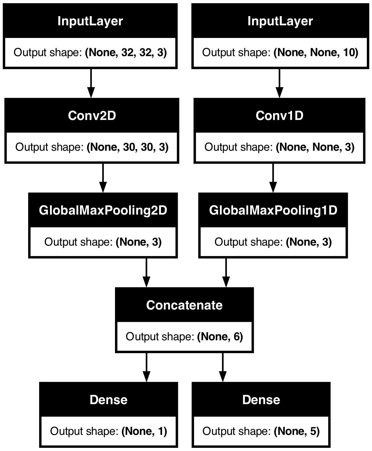
考虑以下模型，它有一个形状为 (32, 32, 3) 的图像输入（即 (高, 宽, 通道)）和一个形状为 (None, 10) 的时间序列输入（即 (时间步, 特征)）。我们的模型将根据这些输入的组合计算出两个输出：一个“分数”（形状为 (1,)）和一个包含五个类别的概率分布（形状为 (5,)）。

image_input = keras.Input(shape=(32, 32, 3), name="img_input")
timeseries_input = keras.Input(shape=(None, 10), name="ts_input")

x1 = layers.Conv2D(3, 3)(image_input)
x1 = layers.GlobalMaxPooling2D()(x1)

x2 = layers.Conv1D(3, 3)(timeseries_input)
x2 = layers.GlobalMaxPooling1D()(x2)

x = layers.concatenate([x1, x2])

score_output = layers.Dense(1, name="score_output")(x)
class_output = layers.Dense(5, name="class_output")(x)

model = keras.Model(
    inputs=[image_input, timeseries_input], outputs=[score_output, class_output]
)

让我们绘制此模型，以便你清楚了解我们在此进行的操作（请注意，图中显示的形状是批次形状，而不是每个样本的形状）。

keras.utils.plot_model(model, "multi_input_and_output_model.png", show_shapes=True)

png

在编译时，我们可以通过将损失函数作为列表传递来为不同的输出指定不同的损失函数。

model.compile(
    optimizer=keras.optimizers.RMSprop(1e-3),
    loss=[
        keras.losses.MeanSquaredError(),
        keras.losses.CategoricalCrossentropy(),
    ],
)

如果我们只向模型传递一个损失函数，则同一个损失函数将被应用于每个输出（这在这里不适用）。

指标也类似。

model.compile(
    optimizer=keras.optimizers.RMSprop(1e-3),
    loss=[
        keras.losses.MeanSquaredError(),
        keras.losses.CategoricalCrossentropy(),
    ],
    metrics=[
        [
            keras.metrics.MeanAbsolutePercentageError(),
            keras.metrics.MeanAbsoluteError(),
        ],
        [keras.metrics.CategoricalAccuracy()],
    ],
)

由于我们给输出层指定了名称，也可以通过字典来指定每个输出的损失和指标。

model.compile(
    optimizer=keras.optimizers.RMSprop(1e-3),
    loss={
        "score_output": keras.losses.MeanSquaredError(),
        "class_output": keras.losses.CategoricalCrossentropy(),
    },
    metrics={
        "score_output": [
            keras.metrics.MeanAbsolutePercentageError(),
            keras.metrics.MeanAbsoluteError(),
        ],
        "class_output": [keras.metrics.CategoricalAccuracy()],
    },
)

如果输出超过 2 个，我们建议使用明确的名称和字典。

可以使用 loss_weights 参数为不同输出的损失赋予不同的权重（例如，在我们的示例中，可能希望更侧重于“分数”损失，使其重要性是类别损失的 2 倍）。

model.compile(
    optimizer=keras.optimizers.RMSprop(1e-3),
    loss={
        "score_output": keras.losses.MeanSquaredError(),
        "class_output": keras.losses.CategoricalCrossentropy(),
    },
    metrics={
        "score_output": [
            keras.metrics.MeanAbsolutePercentageError(),
            keras.metrics.MeanAbsoluteError(),
        ],
        "class_output": [keras.metrics.CategoricalAccuracy()],
    },
    loss_weights={"score_output": 2.0, "class_output": 1.0},
)

如果某些输出仅用于预测而非训练，你也可以选择不计算这些输出的损失。

# List loss version
model.compile(
    optimizer=keras.optimizers.RMSprop(1e-3),
    loss=[None, keras.losses.CategoricalCrossentropy()],
)

# Or dict loss version
model.compile(
    optimizer=keras.optimizers.RMSprop(1e-3),
    loss={"class_output": keras.losses.CategoricalCrossentropy()},
)

在 fit() 中将数据传递给多输入或多输出模型的方式类似于在 compile 中指定损失函数：你可以传递**NumPy 数组列表**（与接收损失函数的输出一一对应）或**将输出名称映射到 NumPy 数组的字典**。

model.compile(
    optimizer=keras.optimizers.RMSprop(1e-3),
    loss=[
        keras.losses.MeanSquaredError(),
        keras.losses.CategoricalCrossentropy(),
    ],
)

# Generate dummy NumPy data
img_data = np.random.random_sample(size=(100, 32, 32, 3))
ts_data = np.random.random_sample(size=(100, 20, 10))
score_targets = np.random.random_sample(size=(100, 1))
class_targets = np.random.random_sample(size=(100, 5))

# Fit on lists
model.fit([img_data, ts_data], [score_targets, class_targets], batch_size=32, epochs=1)

# Alternatively, fit on dicts
model.fit(
    {"img_input": img_data, "ts_input": ts_data},
    {"score_output": score_targets, "class_output": class_targets},
    batch_size=32,
    epochs=1,
)

 4/4 ━━━━━━━━━━━━━━━━━━━━ 0s 62ms/step - loss: 18.0146
 4/4 ━━━━━━━━━━━━━━━━━━━━ 0s 56ms/step - loss: 17.6494

<keras.src.callbacks.history.History at 0x31a6c5810>

这是一个 Dataset 的使用示例：类似于 NumPy 数组，Dataset 应返回一个字典元组。

train_dataset = tf.data.Dataset.from_tensor_slices(
    (
        {"img_input": img_data, "ts_input": ts_data},
        {"score_output": score_targets, "class_output": class_targets},
    )
)
train_dataset = train_dataset.shuffle(buffer_size=1024).batch(64)

model.fit(train_dataset, epochs=1)

 2/2 ━━━━━━━━━━━━━━━━━━━━ 0s 197ms/step - loss: 17.8578

<keras.src.callbacks.history.History at 0x17c7e5690>

使用回调

Keras 中的回调是在训练期间不同点（例如，epoch 开始时、批次结束时、epoch 结束时等）被调用的对象。它们可以用于实现某些行为，例如：

在训练期间的不同时间点进行验证（超出内置的每 epoch 验证）
定期或当模型超过某个准确率阈值时保存检查点
当训练似乎停滞不前时改变模型的学习率
当训练似乎停滞不前时对顶层进行微调
在训练结束或达到某个性能阈值时发送电子邮件或即时消息通知
等等。

回调可以作为列表传递给你的 fit() 调用。

model = get_compiled_model()

callbacks = [
    keras.callbacks.EarlyStopping(
        # Stop training when `val_loss` is no longer improving
        monitor="val_loss",
        # "no longer improving" being defined as "no better than 1e-2 less"
        min_delta=1e-2,
        # "no longer improving" being further defined as "for at least 2 epochs"
        patience=2,
        verbose=1,
    )
]
model.fit(
    x_train,
    y_train,
    epochs=20,
    batch_size=64,
    callbacks=callbacks,
    validation_split=0.2,
)

Epoch 1/20
 625/625 ━━━━━━━━━━━━━━━━━━━━ 1s 622us/step - loss: 0.6245 - sparse_categorical_accuracy: 0.8275 - val_loss: 0.2231 - val_sparse_categorical_accuracy: 0.9330
Epoch 2/20
 625/625 ━━━━━━━━━━━━━━━━━━━━ 0s 404us/step - loss: 0.1809 - sparse_categorical_accuracy: 0.9460 - val_loss: 0.1727 - val_sparse_categorical_accuracy: 0.9476
Epoch 3/20
 625/625 ━━━━━━━━━━━━━━━━━━━━ 0s 398us/step - loss: 0.1336 - sparse_categorical_accuracy: 0.9598 - val_loss: 0.1564 - val_sparse_categorical_accuracy: 0.9545
Epoch 4/20
 625/625 ━━━━━━━━━━━━━━━━━━━━ 0s 400us/step - loss: 0.1012 - sparse_categorical_accuracy: 0.9699 - val_loss: 0.1502 - val_sparse_categorical_accuracy: 0.9570
Epoch 5/20
 625/625 ━━━━━━━━━━━━━━━━━━━━ 0s 403us/step - loss: 0.0835 - sparse_categorical_accuracy: 0.9748 - val_loss: 0.1436 - val_sparse_categorical_accuracy: 0.9589
Epoch 6/20
 625/625 ━━━━━━━━━━━━━━━━━━━━ 0s 396us/step - loss: 0.0699 - sparse_categorical_accuracy: 0.9783 - val_loss: 0.1484 - val_sparse_categorical_accuracy: 0.9577
Epoch 7/20
 625/625 ━━━━━━━━━━━━━━━━━━━━ 0s 402us/step - loss: 0.0603 - sparse_categorical_accuracy: 0.9814 - val_loss: 0.1406 - val_sparse_categorical_accuracy: 0.9629
Epoch 7: early stopping

<keras.src.callbacks.history.History at 0x31ae37c10>

许多内置回调可用

Keras 中已有很多内置回调可用，例如：

ModelCheckpoint：周期性保存模型。
EarlyStopping：当训练不再改进验证指标时停止训练。
TensorBoard：周期性写入模型日志，可在 TensorBoard 中可视化（更多详情请参阅“可视化”部分）。
CSVLogger：将损失和指标数据流式传输到 CSV 文件。
等。

有关完整列表，请参阅 callbacks 文档。

编写自己的回调

你可以通过继承基类 keras.callbacks.Callback 创建自定义回调。回调可以通过类属性 self.model 访问其关联的模型。

请务必阅读编写自定义回调的完整指南。

这是一个简单的示例，用于在训练期间保存每批次的损失值列表。

class LossHistory(keras.callbacks.Callback):
    def on_train_begin(self, logs):
        self.per_batch_losses = []

    def on_batch_end(self, batch, logs):
        self.per_batch_losses.append(logs.get("loss"))

模型检查点

当你在相对较大的数据集上训练模型时，定期保存模型的检查点至关重要。

实现此目的最简单的方法是使用 ModelCheckpoint 回调。

model = get_compiled_model()

callbacks = [
    keras.callbacks.ModelCheckpoint(
        # Path where to save the model
        # The two parameters below mean that we will overwrite
        # the current checkpoint if and only if
        # the `val_loss` score has improved.
        # The saved model name will include the current epoch.
        filepath="mymodel_{epoch}.keras",
        save_best_only=True,  # Only save a model if `val_loss` has improved.
        monitor="val_loss",
        verbose=1,
    )
]
model.fit(
    x_train,
    y_train,
    epochs=2,
    batch_size=64,
    callbacks=callbacks,
    validation_split=0.2,
)

Epoch 1/2
 559/625 ━━━━━━━━━━━━━━━━━[37m━━━  0s 360us/step - loss: 0.6490 - sparse_categorical_accuracy: 0.8209
Epoch 1: val_loss improved from inf to 0.22393, saving model to mymodel_1.keras
 625/625 ━━━━━━━━━━━━━━━━━━━━ 1s 577us/step - loss: 0.6194 - sparse_categorical_accuracy: 0.8289 - val_loss: 0.2239 - val_sparse_categorical_accuracy: 0.9340
Epoch 2/2
 565/625 ━━━━━━━━━━━━━━━━━━[37m━━  0s 355us/step - loss: 0.1816 - sparse_categorical_accuracy: 0.9476
Epoch 2: val_loss improved from 0.22393 to 0.16868, saving model to mymodel_2.keras
 625/625 ━━━━━━━━━━━━━━━━━━━━ 0s 411us/step - loss: 0.1806 - sparse_categorical_accuracy: 0.9479 - val_loss: 0.1687 - val_sparse_categorical_accuracy: 0.9494

<keras.src.callbacks.history.History at 0x2e5cb7250>

ModelCheckpoint 回调可用于实现容错：在训练意外中断的情况下，能够从模型最后保存的状态重新启动训练。这是一个基本示例：

# Prepare a directory to store all the checkpoints.
checkpoint_dir = "./ckpt"
if not os.path.exists(checkpoint_dir):
    os.makedirs(checkpoint_dir)


def make_or_restore_model():
    # Either restore the latest model, or create a fresh one
    # if there is no checkpoint available.
    checkpoints = [checkpoint_dir + "/" + name for name in os.listdir(checkpoint_dir)]
    if checkpoints:
        latest_checkpoint = max(checkpoints, key=os.path.getctime)
        print("Restoring from", latest_checkpoint)
        return keras.models.load_model(latest_checkpoint)
    print("Creating a new model")
    return get_compiled_model()


model = make_or_restore_model()
callbacks = [
    # This callback saves the model every 100 batches.
    # We include the training loss in the saved model name.
    keras.callbacks.ModelCheckpoint(
        filepath=checkpoint_dir + "/model-loss={loss:.2f}.keras", save_freq=100
    )
]
model.fit(x_train, y_train, epochs=1, callbacks=callbacks)

Creating a new model
 1563/1563 ━━━━━━━━━━━━━━━━━━━━ 1s 390us/step - loss: 0.4910 - sparse_categorical_accuracy: 0.8623

<keras.src.callbacks.history.History at 0x2e5c454e0>

你也可以编写自己的回调来保存和恢复模型。

关于序列化和保存的完整指南，请参阅保存和序列化模型指南。

使用学习率调度

训练深度学习模型时的一个常见模式是随着训练的进行逐渐降低学习率。这通常被称为“学习率衰减”。

学习率衰减调度可以是静态的（提前固定，作为当前 epoch 或当前批次索引的函数），也可以是动态的（响应模型的当前行为，特别是验证损失）。

将调度传递给优化器

通过在优化器中将调度对象作为 learning_rate 参数传递，可以轻松使用静态学习率衰减调度。

initial_learning_rate = 0.1
lr_schedule = keras.optimizers.schedules.ExponentialDecay(
    initial_learning_rate, decay_steps=100000, decay_rate=0.96, staircase=True
)

optimizer = keras.optimizers.RMSprop(learning_rate=lr_schedule)

有几种内置调度可用：ExponentialDecay, PiecewiseConstantDecay, PolynomialDecay, 和 InverseTimeDecay。

使用回调实现动态学习率调度

使用这些调度对象无法实现动态学习率调度（例如，当验证损失不再改善时降低学习率），因为优化器无法访问验证指标。

然而，回调可以访问所有指标，包括验证指标！因此，你可以通过使用一个修改优化器当前学习率的回调来实现此模式。事实上，这甚至作为 ReduceLROnPlateau 回调内置在 Keras 中。

使用 TensorBoard 可视化训练期间的损失和指标

在训练期间监控模型的最佳方式是使用 TensorBoard – 一个可以在本地运行的基于浏览器的应用程序，它为你提供了：

训练和评估损失与指标的实时图表
（可选）你的层激活直方图可视化
（可选）你的 Embedding 层学习到的嵌入空间的 3D 可视化

如果你使用 pip 安装了 TensorFlow，应该可以从命令行启动 TensorBoard。

tensorboard --logdir=/full_path_to_your_logs

使用 TensorBoard 回调

使用 Keras 模型和 fit() 方法与 TensorBoard 结合使用的最简单方法是使用 TensorBoard 回调。

在最简单的情况下，只需指定回调应写入日志的位置，即可开始使用：

keras.callbacks.TensorBoard(
    log_dir="/full_path_to_your_logs",
    histogram_freq=0,  # How often to log histogram visualizations
    embeddings_freq=0,  # How often to log embedding visualizations
    update_freq="epoch",
)  # How often to write logs (default: once per epoch)

<keras.src.callbacks.tensorboard.TensorBoard at 0x31b0188b0>

更多信息请参阅 TensorBoard 回调文档。

使用内置方法进行训练与评估

设置

介绍

API 概览：第一个端到端示例

compile() 方法：指定损失函数、指标和优化器

许多内置的优化器、损失函数和指标可用

自定义损失函数

自定义指标

处理不符合标准签名的损失函数和指标

自动划分验证保留集

使用 tf.data Dataset 进行训练与评估

使用 PyDataset 实例进行训练与评估

使用 PyTorch DataLoader 对象进行训练与评估

使用样本权重和类别权重

类别权重

样本权重

将数据传递给多输入、多输出模型

使用回调

许多内置回调可用

编写自己的回调

模型检查点

使用学习率调度

将调度传递给优化器

使用回调实现动态学习率调度

使用 TensorBoard 可视化训练期间的损失和指标

使用 TensorBoard 回调

使用内置方法进行训练与评估

设置

介绍

API 概览：第一个端到端示例

compile() 方法：指定损失函数、指标和优化器

许多内置的优化器、损失函数和指标可用

自定义损失函数

自定义指标

处理不符合标准签名的损失函数和指标

自动划分验证保留集

使用 tf.data Dataset 进行训练与评估

使用 PyDataset 实例进行训练与评估

使用 PyTorch DataLoader 对象进行训练与评估

使用样本权重和类别权重

类别权重

样本权重

将数据传递给多输入、多输出模型

使用回调

许多内置回调可用

编写自己的回调

模型检查点

使用学习率调度

将调度传递给优化器

使用回调实现动态学习率调度

使用 TensorBoard 可视化训练期间的损失和指标

使用 TensorBoard 回调

`compile()` 方法：指定损失函数、指标和优化器

使用 `tf.data` Dataset 进行训练与评估

使用 `PyDataset` 实例进行训练与评估

使用 PyTorch `DataLoader` 对象进行训练与评估