函数式 API
作者: fchollet
创建日期 2019/03/01
最后修改日期 2023/06/25
描述: 函数式 API 的完整指南。

设置
import numpy as np
import keras
from keras import layers
from keras import ops
引言
Keras 的*函数式 API* 是一种创建模型的方式,它比 keras.Sequential API 更灵活。函数式 API 可以处理具有非线性拓扑、共享层,甚至多个输入或输出的模型。
主要思想是,深度学习模型通常是一个有向无环图(DAG)的层。因此,函数式 API 是一种构建*层图*的方式。
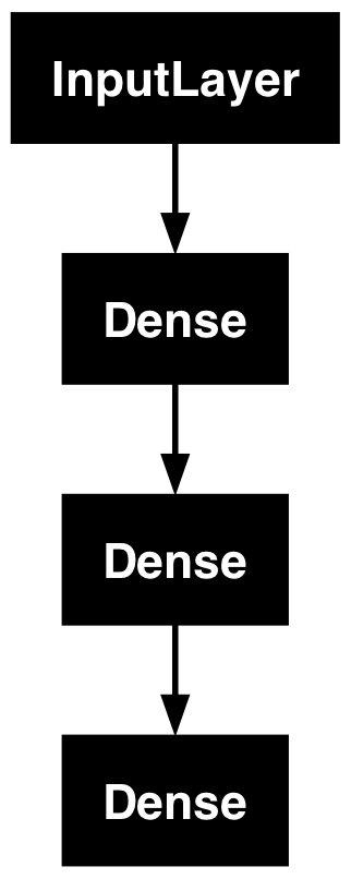
考虑以下模型
(input: 784-dimensional vectors)
       ↧
[Dense (64 units, relu activation)]
       ↧
[Dense (64 units, relu activation)]
       ↧
[Dense (10 units, softmax activation)]
       ↧
(output: logits of a probability distribution over 10 classes)
这是一个包含三个基本层的图。要使用函数式 API 构建此模型,首先创建一个输入节点
inputs = keras.Input(shape=(784,))
数据形状设置为 784 维向量。批次大小总是被省略,因为只指定了每个样本的形状。
例如,如果您有一个形状为 (32, 32, 3) 的图像输入,您将使用
# Just for demonstration purposes.
img_inputs = keras.Input(shape=(32, 32, 3))
返回的 inputs 包含您馈送到模型中的输入数据的形状和 dtype 的信息。形状如下
inputs.shape
(None, 784)
数据类型如下
inputs.dtype
'float32'
通过在此 inputs 对象上调用一个层,您可以在层图中创建一个新节点
dense = layers.Dense(64, activation="relu")
x = dense(inputs)
“层调用”操作就像从“inputs”到您创建的这个层绘制箭头一样。您正在将输入“传递”给 dense 层,并将 x 作为输出获取。
让我们在层图中添加更多层
x = layers.Dense(64, activation="relu")(x)
outputs = layers.Dense(10)(x)
此时,您可以通过在层图中指定模型的输入和输出,来创建 Model
model = keras.Model(inputs=inputs, outputs=outputs, name="mnist_model")
让我们看看模型摘要是什么样的
model.summary()
Model: "mnist_model"
┏━━━━━━━━━━━━━━━━━━━━━━━━━━━━━━━━━┳━━━━━━━━━━━━━━━━━━━━━━━━┳━━━━━━━━━━━━━━━┓
┃ Layer (type)                    ┃ Output Shape           ┃       Param # ┃
┡━━━━━━━━━━━━━━━━━━━━━━━━━━━━━━━━━╇━━━━━━━━━━━━━━━━━━━━━━━━╇━━━━━━━━━━━━━━━┩
│ input_layer (InputLayer)        │ (None, 784)            │             0 │
├─────────────────────────────────┼────────────────────────┼───────────────┤
│ dense (Dense)                   │ (None, 64)             │        50,240 │
├─────────────────────────────────┼────────────────────────┼───────────────┤
│ dense_1 (Dense)                 │ (None, 64)             │         4,160 │
├─────────────────────────────────┼────────────────────────┼───────────────┤
│ dense_2 (Dense)                 │ (None, 10)             │           650 │
└─────────────────────────────────┴────────────────────────┴───────────────┘
Total params: 55,050 (215.04 KB)
Trainable params: 55,050 (215.04 KB)
Non-trainable params: 0 (0.00 B)
您还可以将模型绘制成图
keras.utils.plot_model(model, "my_first_model.png")
此外,您可以选择在绘制的图中显示每个层的输入和输出形状
keras.utils.plot_model(model, "my_first_model_with_shape_info.png", show_shapes=True)
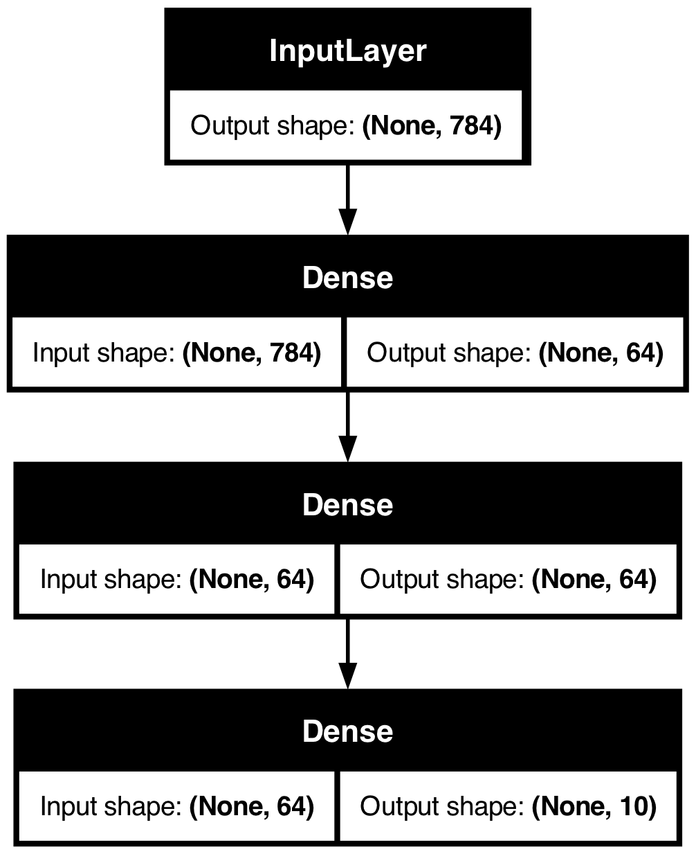
此图和代码几乎完全相同。在代码版本中,连接箭头被调用操作取代。
“层图”是深度学习模型的直观心智图,而函数式 API 是一种创建模型的方式,它密切地反映了这一点。
训练、评估和推断
使用函数式 API 构建的模型,其训练、评估和推断方式与 Sequential 模型完全相同。
Model 类提供了内置的训练循环(fit() 方法)和内置的评估循环(evaluate() 方法)。请注意,您可以轻松定制这些循环来实现您自己的训练例程。另请参阅关于定制 fit() 中发生的行为的指南
在这里,加载 MNIST 图像数据,将其重塑为向量,在数据上拟合模型(同时监控验证分割上的性能),然后在测试数据上评估模型
(x_train, y_train), (x_test, y_test) = keras.datasets.mnist.load_data()

x_train = x_train.reshape(60000, 784).astype("float32") / 255
x_test = x_test.reshape(10000, 784).astype("float32") / 255

model.compile(
    loss=keras.losses.SparseCategoricalCrossentropy(from_logits=True),
    optimizer=keras.optimizers.RMSprop(),
    metrics=["accuracy"],
)

history = model.fit(x_train, y_train, batch_size=64, epochs=2, validation_split=0.2)

test_scores = model.evaluate(x_test, y_test, verbose=2)
print("Test loss:", test_scores[0])
print("Test accuracy:", test_scores[1])
Epoch 1/2
 750/750 ━━━━━━━━━━━━━━━━━━━━ 1s 863us/step - accuracy: 0.8425 - loss: 0.5733 - val_accuracy: 0.9496 - val_loss: 0.1711
Epoch 2/2
 750/750 ━━━━━━━━━━━━━━━━━━━━ 1s 859us/step - accuracy: 0.9509 - loss: 0.1641 - val_accuracy: 0.9578 - val_loss: 0.1396
313/313 - 0s - 341us/step - accuracy: 0.9613 - loss: 0.1288
Test loss: 0.12876172363758087
Test accuracy: 0.9613000154495239
如需进一步阅读,请参阅训练和评估指南。
保存和序列化
使用函数式 API 构建的模型,其保存和序列化方式与 Sequential 模型相同。保存函数式模型的标准方法是调用 model.save() 将整个模型保存为一个文件。即使构建模型的代码不再可用,您稍后也可以从此文件重新创建相同的模型。
此保存的文件包含: - 模型架构 - 模型权重值(在训练期间学习到的) - 模型训练配置(如果存在,如传递给 compile() 的) - 优化器及其状态(如果存在,以便从中断处继续训练)
model.save("my_model.keras")
del model
# Recreate the exact same model purely from the file:
model = keras.models.load_model("my_model.keras")
有关详细信息,请阅读模型序列化和保存指南。
使用相同的层图定义多个模型
在函数式 API 中,通过在层图中指定模型的输入和输出,来创建模型。这意味着单个层图可以用于生成多个模型。
在下面的示例中,您使用相同的层堆栈实例化两个模型:一个 encoder 模型将图像输入转换为 16 维向量,以及一个用于训练的端到端 autoencoder 模型。
encoder_input = keras.Input(shape=(28, 28, 1), name="img")
x = layers.Conv2D(16, 3, activation="relu")(encoder_input)
x = layers.Conv2D(32, 3, activation="relu")(x)
x = layers.MaxPooling2D(3)(x)
x = layers.Conv2D(32, 3, activation="relu")(x)
x = layers.Conv2D(16, 3, activation="relu")(x)
encoder_output = layers.GlobalMaxPooling2D()(x)

encoder = keras.Model(encoder_input, encoder_output, name="encoder")
encoder.summary()

x = layers.Reshape((4, 4, 1))(encoder_output)
x = layers.Conv2DTranspose(16, 3, activation="relu")(x)
x = layers.Conv2DTranspose(32, 3, activation="relu")(x)
x = layers.UpSampling2D(3)(x)
x = layers.Conv2DTranspose(16, 3, activation="relu")(x)
decoder_output = layers.Conv2DTranspose(1, 3, activation="relu")(x)

autoencoder = keras.Model(encoder_input, decoder_output, name="autoencoder")
autoencoder.summary()
Model: "encoder"
┏━━━━━━━━━━━━━━━━━━━━━━━━━━━━━━━━━┳━━━━━━━━━━━━━━━━━━━━━━━━┳━━━━━━━━━━━━━━━┓
┃ Layer (type)                    ┃ Output Shape           ┃       Param # ┃
┡━━━━━━━━━━━━━━━━━━━━━━━━━━━━━━━━━╇━━━━━━━━━━━━━━━━━━━━━━━━╇━━━━━━━━━━━━━━━┩
│ img (InputLayer)                │ (None, 28, 28, 1)      │             0 │
├─────────────────────────────────┼────────────────────────┼───────────────┤
│ conv2d (Conv2D)                 │ (None, 26, 26, 16)     │           160 │
├─────────────────────────────────┼────────────────────────┼───────────────┤
│ conv2d_1 (Conv2D)               │ (None, 24, 24, 32)     │         4,640 │
├─────────────────────────────────┼────────────────────────┼───────────────┤
│ max_pooling2d (MaxPooling2D)    │ (None, 8, 8, 32)       │             0 │
├─────────────────────────────────┼────────────────────────┼───────────────┤
│ conv2d_2 (Conv2D)               │ (None, 6, 6, 32)       │         9,248 │
├─────────────────────────────────┼────────────────────────┼───────────────┤
│ conv2d_3 (Conv2D)               │ (None, 4, 4, 16)       │         4,624 │
├─────────────────────────────────┼────────────────────────┼───────────────┤
│ global_max_pooling2d            │ (None, 16)             │             0 │
│ (GlobalMaxPooling2D)            │                        │               │
└─────────────────────────────────┴────────────────────────┴───────────────┘
Total params: 18,672 (72.94 KB)
Trainable params: 18,672 (72.94 KB)
Non-trainable params: 0 (0.00 B)
Model: "autoencoder"
┏━━━━━━━━━━━━━━━━━━━━━━━━━━━━━━━━━┳━━━━━━━━━━━━━━━━━━━━━━━━┳━━━━━━━━━━━━━━━┓
┃ Layer (type)                    ┃ Output Shape           ┃       Param # ┃
┡━━━━━━━━━━━━━━━━━━━━━━━━━━━━━━━━━╇━━━━━━━━━━━━━━━━━━━━━━━━╇━━━━━━━━━━━━━━━┩
│ img (InputLayer)                │ (None, 28, 28, 1)      │             0 │
├─────────────────────────────────┼────────────────────────┼───────────────┤
│ conv2d (Conv2D)                 │ (None, 26, 26, 16)     │           160 │
├─────────────────────────────────┼────────────────────────┼───────────────┤
│ conv2d_1 (Conv2D)               │ (None, 24, 24, 32)     │         4,640 │
├─────────────────────────────────┼────────────────────────┼───────────────┤
│ max_pooling2d (MaxPooling2D)    │ (None, 8, 8, 32)       │             0 │
├─────────────────────────────────┼────────────────────────┼───────────────┤
│ conv2d_2 (Conv2D)               │ (None, 6, 6, 32)       │         9,248 │
├─────────────────────────────────┼────────────────────────┼───────────────┤
│ conv2d_3 (Conv2D)               │ (None, 4, 4, 16)       │         4,624 │
├─────────────────────────────────┼────────────────────────┼───────────────┤
│ global_max_pooling2d            │ (None, 16)             │             0 │
│ (GlobalMaxPooling2D)            │                        │               │
├─────────────────────────────────┼────────────────────────┼───────────────┤
│ reshape (Reshape)               │ (None, 4, 4, 1)        │             0 │
├─────────────────────────────────┼────────────────────────┼───────────────┤
│ conv2d_transpose                │ (None, 6, 6, 16)       │           160 │
│ (Conv2DTranspose)               │                        │               │
├─────────────────────────────────┼────────────────────────┼───────────────┤
│ conv2d_transpose_1              │ (None, 8, 8, 32)       │         4,640 │
│ (Conv2DTranspose)               │                        │               │
├─────────────────────────────────┼────────────────────────┼───────────────┤
│ up_sampling2d (UpSampling2D)    │ (None, 24, 24, 32)     │             0 │
├─────────────────────────────────┼────────────────────────┼───────────────┤
│ conv2d_transpose_2              │ (None, 26, 26, 16)     │         4,624 │
│ (Conv2DTranspose)               │                        │               │
├─────────────────────────────────┼────────────────────────┼───────────────┤
│ conv2d_transpose_3              │ (None, 28, 28, 1)      │           145 │
│ (Conv2DTranspose)               │                        │               │
└─────────────────────────────────┴────────────────────────┴───────────────┘
Total params: 28,241 (110.32 KB)
Trainable params: 28,241 (110.32 KB)
Non-trainable params: 0 (0.00 B)
在这里,解码架构与编码架构严格对称,因此输出形状与输入形状 (28, 28, 1) 相同。
Conv2D 层的反向是 Conv2DTranspose 层,而 MaxPooling2D 层的反向是 UpSampling2D 层。
所有模型都像层一样可调用
您可以在 Input 对象或另一个层的输出上调用任何模型,就像它是层一样。通过调用模型,您不仅重用了模型的架构,还重用了其权重。
为了看到它的实际应用,这里是自编码器示例的另一种实现方式,它创建一个编码器模型和一个解码器模型,然后通过两次调用将它们链接起来以获得自编码器模型
encoder_input = keras.Input(shape=(28, 28, 1), name="original_img")
x = layers.Conv2D(16, 3, activation="relu")(encoder_input)
x = layers.Conv2D(32, 3, activation="relu")(x)
x = layers.MaxPooling2D(3)(x)
x = layers.Conv2D(32, 3, activation="relu")(x)
x = layers.Conv2D(16, 3, activation="relu")(x)
encoder_output = layers.GlobalMaxPooling2D()(x)

encoder = keras.Model(encoder_input, encoder_output, name="encoder")
encoder.summary()

decoder_input = keras.Input(shape=(16,), name="encoded_img")
x = layers.Reshape((4, 4, 1))(decoder_input)
x = layers.Conv2DTranspose(16, 3, activation="relu")(x)
x = layers.Conv2DTranspose(32, 3, activation="relu")(x)
x = layers.UpSampling2D(3)(x)
x = layers.Conv2DTranspose(16, 3, activation="relu")(x)
decoder_output = layers.Conv2DTranspose(1, 3, activation="relu")(x)

decoder = keras.Model(decoder_input, decoder_output, name="decoder")
decoder.summary()

autoencoder_input = keras.Input(shape=(28, 28, 1), name="img")
encoded_img = encoder(autoencoder_input)
decoded_img = decoder(encoded_img)
autoencoder = keras.Model(autoencoder_input, decoded_img, name="autoencoder")
autoencoder.summary()
Model: "encoder"
┏━━━━━━━━━━━━━━━━━━━━━━━━━━━━━━━━━┳━━━━━━━━━━━━━━━━━━━━━━━━┳━━━━━━━━━━━━━━━┓
┃ Layer (type)                    ┃ Output Shape           ┃       Param # ┃
┡━━━━━━━━━━━━━━━━━━━━━━━━━━━━━━━━━╇━━━━━━━━━━━━━━━━━━━━━━━━╇━━━━━━━━━━━━━━━┩
│ original_img (InputLayer)       │ (None, 28, 28, 1)      │             0 │
├─────────────────────────────────┼────────────────────────┼───────────────┤
│ conv2d_4 (Conv2D)               │ (None, 26, 26, 16)     │           160 │
├─────────────────────────────────┼────────────────────────┼───────────────┤
│ conv2d_5 (Conv2D)               │ (None, 24, 24, 32)     │         4,640 │
├─────────────────────────────────┼────────────────────────┼───────────────┤
│ max_pooling2d_1 (MaxPooling2D)  │ (None, 8, 8, 32)       │             0 │
├─────────────────────────────────┼────────────────────────┼───────────────┤
│ conv2d_6 (Conv2D)               │ (None, 6, 6, 32)       │         9,248 │
├─────────────────────────────────┼────────────────────────┼───────────────┤
│ conv2d_7 (Conv2D)               │ (None, 4, 4, 16)       │         4,624 │
├─────────────────────────────────┼────────────────────────┼───────────────┤
│ global_max_pooling2d_1          │ (None, 16)             │             0 │
│ (GlobalMaxPooling2D)            │                        │               │
└─────────────────────────────────┴────────────────────────┴───────────────┘
Total params: 18,672 (72.94 KB)
Trainable params: 18,672 (72.94 KB)
Non-trainable params: 0 (0.00 B)
Model: "decoder"
┏━━━━━━━━━━━━━━━━━━━━━━━━━━━━━━━━━┳━━━━━━━━━━━━━━━━━━━━━━━━┳━━━━━━━━━━━━━━━┓
┃ Layer (type)                    ┃ Output Shape           ┃       Param # ┃
┡━━━━━━━━━━━━━━━━━━━━━━━━━━━━━━━━━╇━━━━━━━━━━━━━━━━━━━━━━━━╇━━━━━━━━━━━━━━━┩
│ encoded_img (InputLayer)        │ (None, 16)             │             0 │
├─────────────────────────────────┼────────────────────────┼───────────────┤
│ reshape_1 (Reshape)             │ (None, 4, 4, 1)        │             0 │
├─────────────────────────────────┼────────────────────────┼───────────────┤
│ conv2d_transpose_4              │ (None, 6, 6, 16)       │           160 │
│ (Conv2DTranspose)               │                        │               │
├─────────────────────────────────┼────────────────────────┼───────────────┤
│ conv2d_transpose_5              │ (None, 8, 8, 32)       │         4,640 │
│ (Conv2DTranspose)               │                        │               │
├─────────────────────────────────┼────────────────────────┼───────────────┤
│ up_sampling2d_1 (UpSampling2D)  │ (None, 24, 24, 32)     │             0 │
├─────────────────────────────────┼────────────────────────┼───────────────┤
│ conv2d_transpose_6              │ (None, 26, 26, 16)     │         4,624 │
│ (Conv2DTranspose)               │                        │               │
├─────────────────────────────────┼────────────────────────┼───────────────┤
│ conv2d_transpose_7              │ (None, 28, 28, 1)      │           145 │
│ (Conv2DTranspose)               │                        │               │
└─────────────────────────────────┴────────────────────────┴───────────────┘
Total params: 9,569 (37.38 KB)
Trainable params: 9,569 (37.38 KB)
Non-trainable params: 0 (0.00 B)
Model: "autoencoder"
┏━━━━━━━━━━━━━━━━━━━━━━━━━━━━━━━━━┳━━━━━━━━━━━━━━━━━━━━━━━━┳━━━━━━━━━━━━━━━┓
┃ Layer (type)                    ┃ Output Shape           ┃       Param # ┃
┡━━━━━━━━━━━━━━━━━━━━━━━━━━━━━━━━━╇━━━━━━━━━━━━━━━━━━━━━━━━╇━━━━━━━━━━━━━━━┩
│ img (InputLayer)                │ (None, 28, 28, 1)      │             0 │
├─────────────────────────────────┼────────────────────────┼───────────────┤
│ encoder (Functional)            │ (None, 16)             │        18,672 │
├─────────────────────────────────┼────────────────────────┼───────────────┤
│ decoder (Functional)            │ (None, 28, 28, 1)      │         9,569 │
└─────────────────────────────────┴────────────────────────┴───────────────┘
Total params: 28,241 (110.32 KB)
Trainable params: 28,241 (110.32 KB)
Non-trainable params: 0 (0.00 B)
正如您所见,模型可以嵌套:一个模型可以包含子模型(因为模型就像一个层)。模型嵌套的一个常见用例是*集成*。例如,这里是如何将一组模型集成为一个单一模型,该模型对它们的预测进行平均
def get_model():
    inputs = keras.Input(shape=(128,))
    outputs = layers.Dense(1)(inputs)
    return keras.Model(inputs, outputs)


model1 = get_model()
model2 = get_model()
model3 = get_model()

inputs = keras.Input(shape=(128,))
y1 = model1(inputs)
y2 = model2(inputs)
y3 = model3(inputs)
outputs = layers.average([y1, y2, y3])
ensemble_model = keras.Model(inputs=inputs, outputs=outputs)
处理复杂的图拓扑
具有多个输入和输出的模型
函数式 API 使处理多个输入和输出变得容易。这无法通过 Sequential API 处理。
例如,如果您正在构建一个根据优先级对客户问题工单进行排序并将其路由到正确部门的系统,那么模型将有三个输入
- 工单标题(文本输入),
- 工单正文(文本输入),以及
- 用户添加的任何标签(分类输入)
此模型将有两个输出
- 优先级分数(0 到 1 之间的标量 sigmoid 输出),以及
- 应该处理工单的部门(对部门集合的 softmax 输出)。
您可以使用函数式 API 在几行代码中构建此模型
num_tags = 12  # Number of unique issue tags
num_words = 10000  # Size of vocabulary obtained when preprocessing text data
num_departments = 4  # Number of departments for predictions

title_input = keras.Input(
    shape=(None,), name="title"
)  # Variable-length sequence of ints
body_input = keras.Input(shape=(None,), name="body")  # Variable-length sequence of ints
tags_input = keras.Input(
    shape=(num_tags,), name="tags"
)  # Binary vectors of size `num_tags`

# Embed each word in the title into a 64-dimensional vector
title_features = layers.Embedding(num_words, 64)(title_input)
# Embed each word in the text into a 64-dimensional vector
body_features = layers.Embedding(num_words, 64)(body_input)

# Reduce sequence of embedded words in the title into a single 128-dimensional vector
title_features = layers.LSTM(128)(title_features)
# Reduce sequence of embedded words in the body into a single 32-dimensional vector
body_features = layers.LSTM(32)(body_features)

# Merge all available features into a single large vector via concatenation
x = layers.concatenate([title_features, body_features, tags_input])

# Stick a logistic regression for priority prediction on top of the features
priority_pred = layers.Dense(1, name="priority")(x)
# Stick a department classifier on top of the features
department_pred = layers.Dense(num_departments, name="department")(x)

# Instantiate an end-to-end model predicting both priority and department
model = keras.Model(
    inputs=[title_input, body_input, tags_input],
    outputs={"priority": priority_pred, "department": department_pred},
)
现在绘制模型图
keras.utils.plot_model(model, "multi_input_and_output_model.png", show_shapes=True)
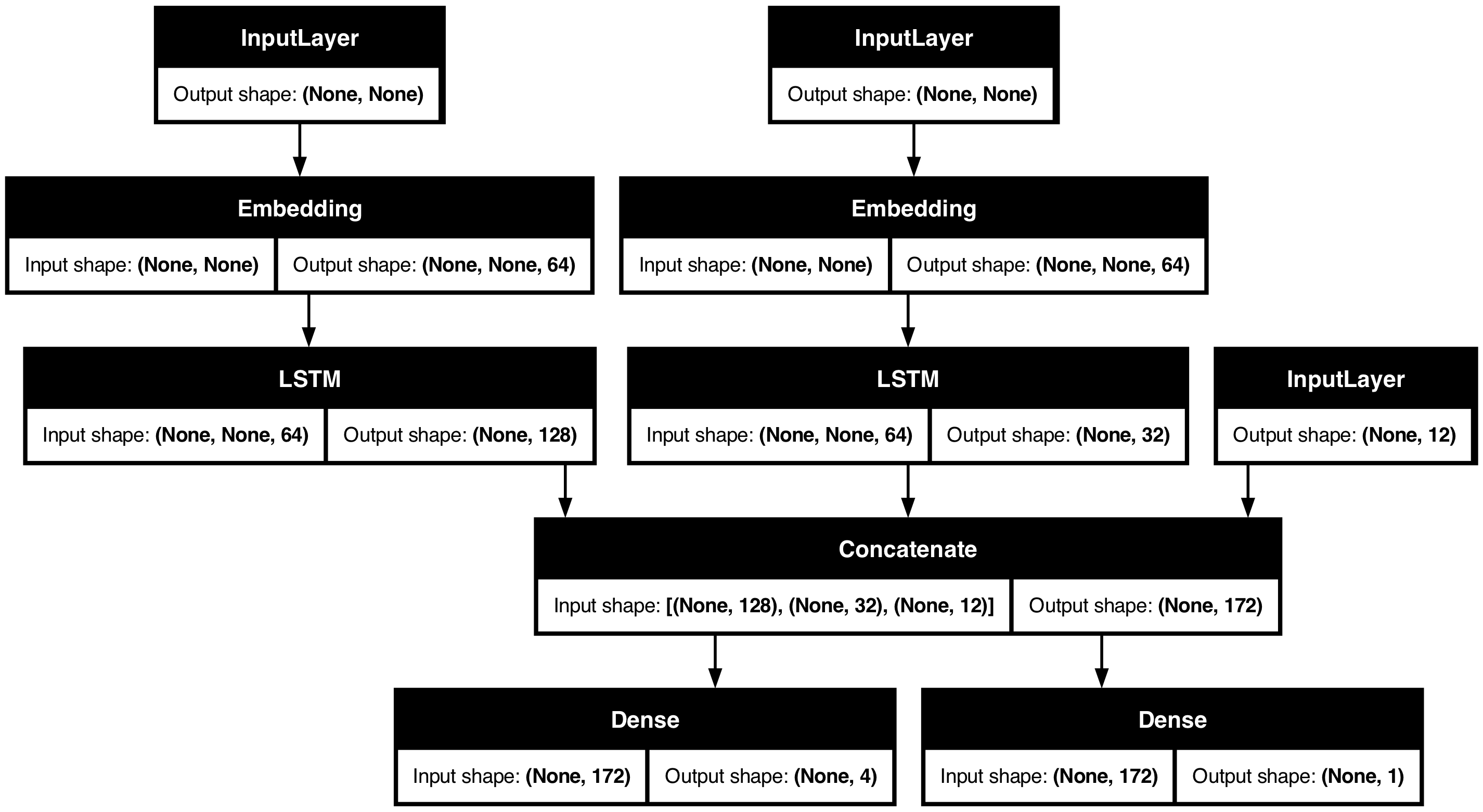
编译此模型时,您可以为每个输出分配不同的损失。您甚至可以为每个损失分配不同的权重,以调节它们对总训练损失的贡献。
model.compile(
    optimizer=keras.optimizers.RMSprop(1e-3),
    loss=[
        keras.losses.BinaryCrossentropy(from_logits=True),
        keras.losses.CategoricalCrossentropy(from_logits=True),
    ],
    loss_weights=[1.0, 0.2],
)
由于输出层有不同的名称,您也可以使用相应的层名称来指定损失和损失权重
model.compile(
    optimizer=keras.optimizers.RMSprop(1e-3),
    loss={
        "priority": keras.losses.BinaryCrossentropy(from_logits=True),
        "department": keras.losses.CategoricalCrossentropy(from_logits=True),
    },
    loss_weights={"priority": 1.0, "department": 0.2},
)
通过传递 NumPy 输入和目标数组列表来训练模型
# Dummy input data
title_data = np.random.randint(num_words, size=(1280, 12))
body_data = np.random.randint(num_words, size=(1280, 100))
tags_data = np.random.randint(2, size=(1280, num_tags)).astype("float32")

# Dummy target data
priority_targets = np.random.random(size=(1280, 1))
dept_targets = np.random.randint(2, size=(1280, num_departments))

model.fit(
    {"title": title_data, "body": body_data, "tags": tags_data},
    {"priority": priority_targets, "department": dept_targets},
    epochs=2,
    batch_size=32,
)
Epoch 1/2
 40/40 ━━━━━━━━━━━━━━━━━━━━ 3s 57ms/step - loss: 1108.3792
Epoch 2/2
 40/40 ━━━━━━━━━━━━━━━━━━━━ 2s 54ms/step - loss: 621.3049

<keras.src.callbacks.history.History at 0x34afc3d90>
使用 Dataset 对象调用 fit 时,它应该生成列表元组,例如 ([title_data, body_data, tags_data], [priority_targets, dept_targets]),或者生成字典元组,例如 ({'title': title_data, 'body': body_data, 'tags': tags_data}, {'priority': priority_targets, 'department': dept_targets})。
有关更详细的解释,请参阅训练和评估指南。
一个玩具 ResNet 模型
除了具有多个输入和输出的模型,函数式 API 还使得处理非线性连接拓扑变得容易——这些模型的层并非按顺序连接,这是 Sequential API 无法处理的。
一个常见的用例是残差连接。让我们构建一个用于 CIFAR10 的玩具 ResNet 模型来演示这一点
inputs = keras.Input(shape=(32, 32, 3), name="img")
x = layers.Conv2D(32, 3, activation="relu")(inputs)
x = layers.Conv2D(64, 3, activation="relu")(x)
block_1_output = layers.MaxPooling2D(3)(x)

x = layers.Conv2D(64, 3, activation="relu", padding="same")(block_1_output)
x = layers.Conv2D(64, 3, activation="relu", padding="same")(x)
block_2_output = layers.add([x, block_1_output])

x = layers.Conv2D(64, 3, activation="relu", padding="same")(block_2_output)
x = layers.Conv2D(64, 3, activation="relu", padding="same")(x)
block_3_output = layers.add([x, block_2_output])

x = layers.Conv2D(64, 3, activation="relu")(block_3_output)
x = layers.GlobalAveragePooling2D()(x)
x = layers.Dense(256, activation="relu")(x)
x = layers.Dropout(0.5)(x)
outputs = layers.Dense(10)(x)

model = keras.Model(inputs, outputs, name="toy_resnet")
model.summary()
Model: "toy_resnet"
┏━━━━━━━━━━━━━━━━━━━━━┳━━━━━━━━━━━━━━━━━━━┳━━━━━━━━━━━━┳━━━━━━━━━━━━━━━━━━━┓
┃ Layer (type)        ┃ Output Shape      ┃    Param # ┃ Connected to      ┃
┡━━━━━━━━━━━━━━━━━━━━━╇━━━━━━━━━━━━━━━━━━━╇━━━━━━━━━━━━╇━━━━━━━━━━━━━━━━━━━┩
│ img (InputLayer)    │ (None, 32, 32, 3) │          0 │ -                 │
├─────────────────────┼───────────────────┼────────────┼───────────────────┤
│ conv2d_8 (Conv2D)   │ (None, 30, 30,    │        896 │ img[0][0]         │
│                     │ 32)               │            │                   │
├─────────────────────┼───────────────────┼────────────┼───────────────────┤
│ conv2d_9 (Conv2D)   │ (None, 28, 28,    │     18,496 │ conv2d_8[0][0]    │
│                     │ 64)               │            │                   │
├─────────────────────┼───────────────────┼────────────┼───────────────────┤
│ max_pooling2d_2     │ (None, 9, 9, 64)  │          0 │ conv2d_9[0][0]    │
│ (MaxPooling2D)      │                   │            │                   │
├─────────────────────┼───────────────────┼────────────┼───────────────────┤
│ conv2d_10 (Conv2D)  │ (None, 9, 9, 64)  │     36,928 │ max_pooling2d_2[… │
├─────────────────────┼───────────────────┼────────────┼───────────────────┤
│ conv2d_11 (Conv2D)  │ (None, 9, 9, 64)  │     36,928 │ conv2d_10[0][0]   │
├─────────────────────┼───────────────────┼────────────┼───────────────────┤
│ add (Add)           │ (None, 9, 9, 64)  │          0 │ conv2d_11[0][0],  │
│                     │                   │            │ max_pooling2d_2[… │
├─────────────────────┼───────────────────┼────────────┼───────────────────┤
│ conv2d_12 (Conv2D)  │ (None, 9, 9, 64)  │     36,928 │ add[0][0]         │
├─────────────────────┼───────────────────┼────────────┼───────────────────┤
│ conv2d_13 (Conv2D)  │ (None, 9, 9, 64)  │     36,928 │ conv2d_12[0][0]   │
├─────────────────────┼───────────────────┼────────────┼───────────────────┤
│ add_1 (Add)         │ (None, 9, 9, 64)  │          0 │ conv2d_13[0][0],  │
│                     │                   │            │ add[0][0]         │
├─────────────────────┼───────────────────┼────────────┼───────────────────┤
│ conv2d_14 (Conv2D)  │ (None, 7, 7, 64)  │     36,928 │ add_1[0][0]       │
├─────────────────────┼───────────────────┼────────────┼───────────────────┤
│ global_average_poo… │ (None, 64)        │          0 │ conv2d_14[0][0]   │
│ (GlobalAveragePool… │                   │            │                   │
├─────────────────────┼───────────────────┼────────────┼───────────────────┤
│ dense_6 (Dense)     │ (None, 256)       │     16,640 │ global_average_p… │
├─────────────────────┼───────────────────┼────────────┼───────────────────┤
│ dropout (Dropout)   │ (None, 256)       │          0 │ dense_6[0][0]     │
├─────────────────────┼───────────────────┼────────────┼───────────────────┤
│ dense_7 (Dense)     │ (None, 10)        │      2,570 │ dropout[0][0]     │
└─────────────────────┴───────────────────┴────────────┴───────────────────┘
Total params: 223,242 (872.04 KB)
Trainable params: 223,242 (872.04 KB)
Non-trainable params: 0 (0.00 B)
绘制模型图
keras.utils.plot_model(model, "mini_resnet.png", show_shapes=True)
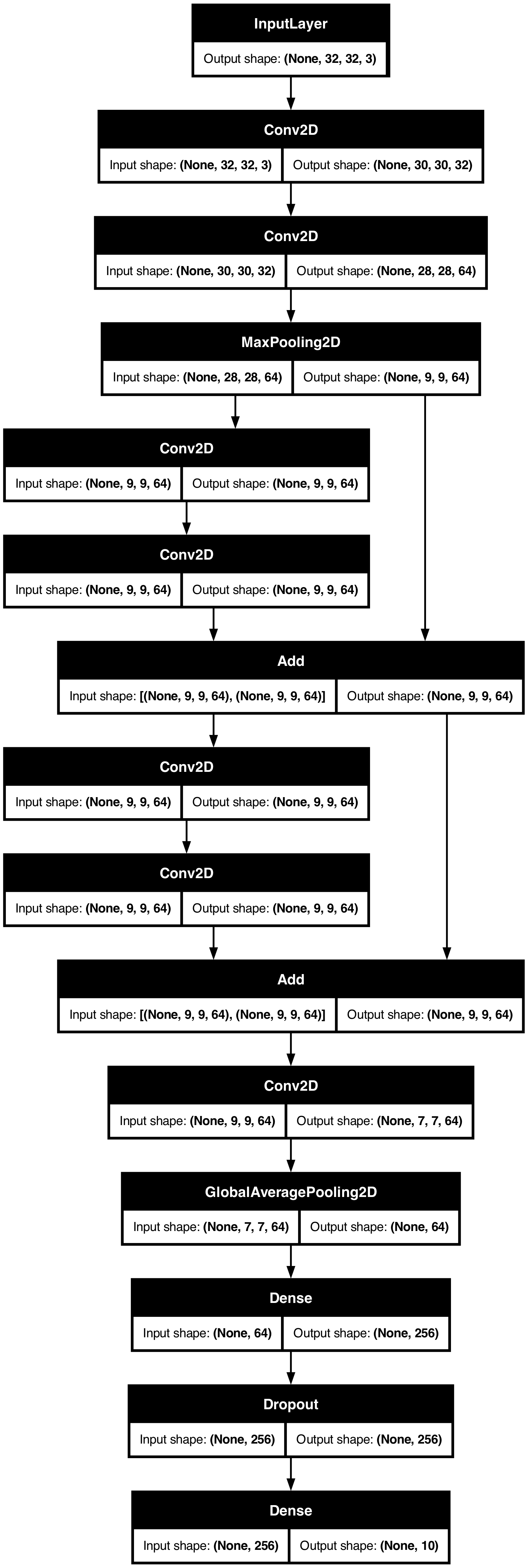
现在训练模型
(x_train, y_train), (x_test, y_test) = keras.datasets.cifar10.load_data()

x_train = x_train.astype("float32") / 255.0
x_test = x_test.astype("float32") / 255.0
y_train = keras.utils.to_categorical(y_train, 10)
y_test = keras.utils.to_categorical(y_test, 10)

model.compile(
    optimizer=keras.optimizers.RMSprop(1e-3),
    loss=keras.losses.CategoricalCrossentropy(from_logits=True),
    metrics=["acc"],
)
# We restrict the data to the first 1000 samples so as to limit execution time
# on Colab. Try to train on the entire dataset until convergence!
model.fit(
    x_train[:1000],
    y_train[:1000],
    batch_size=64,
    epochs=1,
    validation_split=0.2,
)
 13/13 ━━━━━━━━━━━━━━━━━━━━ 1s 60ms/step - acc: 0.1096 - loss: 2.3053 - val_acc: 0.1150 - val_loss: 2.2973

<keras.src.callbacks.history.History at 0x1758bed40>
共享层
函数式 API 的另一个优点是可以使用*共享层*的模型。共享层是在同一个模型中多次重用的层实例——它们学习对应于层图中多个路径的特征。
共享层通常用于对来自相似空间的输入进行编码(例如,两段包含相似词汇的不同文本)。它们使得信息能够在这些不同的输入之间共享,并且可以使用较少的数据来训练这样的模型。如果在其中一个输入中看到了某个词,这将有利于所有通过共享层的输入的处理。
要在函数式 API 中共享一个层,只需多次调用同一个层实例。例如,这里是一个在两个不同文本输入之间共享的 Embedding 层
# Embedding for 1000 unique words mapped to 128-dimensional vectors
shared_embedding = layers.Embedding(1000, 128)

# Variable-length sequence of integers
text_input_a = keras.Input(shape=(None,), dtype="int32")

# Variable-length sequence of integers
text_input_b = keras.Input(shape=(None,), dtype="int32")

# Reuse the same layer to encode both inputs
encoded_input_a = shared_embedding(text_input_a)
encoded_input_b = shared_embedding(text_input_b)
提取和重用层图中的节点
因为您正在操作的层图是一个静态数据结构,所以可以访问和检查它。这就是为什么能够将函数式模型绘制成图像的原因。
这也意味着您可以访问中间层(图中的“节点”)的激活并将其重用于其他地方——这对于特征提取等非常有用。
让我们来看一个例子。这是一个 VGG19 模型,其权重已在 ImageNet 上预训练过
vgg19 = keras.applications.VGG19()
这些是模型的中间层激活,通过查询图数据结构获得
features_list = [layer.output for layer in vgg19.layers]
使用这些特征创建一个新的特征提取模型,该模型返回中间层激活的值
feat_extraction_model = keras.Model(inputs=vgg19.input, outputs=features_list)

img = np.random.random((1, 224, 224, 3)).astype("float32")
extracted_features = feat_extraction_model(img)
这在神经风格迁移等任务中非常方便。
使用自定义层扩展 API
keras 包含多种内置层,例如
- 卷积层:
Conv1D,Conv2D,Conv3D,Conv2DTranspose - 池化层:
MaxPooling1D,MaxPooling2D,MaxPooling3D,AveragePooling1D - RNN 层:
GRU,LSTM,ConvLSTM2D BatchNormalization,Dropout,Embedding等。
但是如果您找不到所需的层,可以通过创建自己的层来轻松扩展 API。所有层都继承自 Layer 类并实现
call方法,指定层执行的计算。build方法,创建层的权重(这只是一种风格约定,因为您也可以在__init__中创建权重)。
要了解如何从头开始创建层,请阅读自定义层和模型指南。
以下是 keras.layers.Dense 的基本实现
class CustomDense(layers.Layer):
    def __init__(self, units=32):
        super().__init__()
        self.units = units

    def build(self, input_shape):
        self.w = self.add_weight(
            shape=(input_shape[-1], self.units),
            initializer="random_normal",
            trainable=True,
        )
        self.b = self.add_weight(
            shape=(self.units,), initializer="random_normal", trainable=True
        )

    def call(self, inputs):
        return ops.matmul(inputs, self.w) + self.b


inputs = keras.Input((4,))
outputs = CustomDense(10)(inputs)

model = keras.Model(inputs, outputs)
为了在自定义层中支持序列化,定义一个 get_config() 方法,该方法返回层实例的构造函数参数
class CustomDense(layers.Layer):
    def __init__(self, units=32):
        super().__init__()
        self.units = units

    def build(self, input_shape):
        self.w = self.add_weight(
            shape=(input_shape[-1], self.units),
            initializer="random_normal",
            trainable=True,
        )
        self.b = self.add_weight(
            shape=(self.units,), initializer="random_normal", trainable=True
        )

    def call(self, inputs):
        return ops.matmul(inputs, self.w) + self.b

    def get_config(self):
        return {"units": self.units}


inputs = keras.Input((4,))
outputs = CustomDense(10)(inputs)

model = keras.Model(inputs, outputs)
config = model.get_config()

new_model = keras.Model.from_config(config, custom_objects={"CustomDense": CustomDense})
可选地,实现类方法 from_config(cls, config),当根据层的配置字典重新创建层实例时会使用此方法。from_config 的默认实现是
def from_config(cls, config):
  return cls(**config)
何时使用函数式 API
您应该使用 Keras 函数式 API 创建新模型,还是直接子类化 Model 类?总的来说,函数式 API 级别更高、更简单、更安全,并且具有子类化模型不支持的一些特性。
然而,当构建不容易表示为有向无环图的层模型时,模型子类化提供了更大的灵活性。例如,您无法使用函数式 API 实现 Tree-RNN,而必须直接子类化 Model。
要深入了解函数式 API 和模型子类化之间的区别,请阅读TensorFlow 2.0 中的符号式 API 和命令式 API 是什么?。
函数式 API 的优势
以下特性对于序贯模型(它们也是数据结构)也适用,但对于子类化模型(它们是 Python 字节码,而非数据结构)则不适用。
更简洁
没有 super().__init__(...),没有 def call(self, ...): 等。
对比
inputs = keras.Input(shape=(32,))
x = layers.Dense(64, activation='relu')(inputs)
outputs = layers.Dense(10)(x)
mlp = keras.Model(inputs, outputs)
与子类化版本对比
class MLP(keras.Model):

  def __init__(self, **kwargs):
    super().__init__(**kwargs)
    self.dense_1 = layers.Dense(64, activation='relu')
    self.dense_2 = layers.Dense(10)

  def call(self, inputs):
    x = self.dense_1(inputs)
    return self.dense_2(x)

# Instantiate the model.
mlp = MLP()
# Necessary to create the model's state.
# The model doesn't have a state until it's called at least once.
_ = mlp(ops.zeros((1, 32)))
定义连接图时进行模型验证
在函数式 API 中,输入规范(形状和数据类型)是提前创建的(使用 Input)。每次调用一个层时,层都会检查传递给它的规范是否与其假设匹配,如果不匹配,则会引发有用的错误消息。
这保证了您可以使用函数式 API 构建的任何模型都可以运行。除了与收敛相关的调试外,所有调试都在模型构建期间静态发生,而不是在执行时。这类似于编译器中的类型检查。
函数式模型可绘制且可检查
您可以将模型绘制成图,并且可以轻松访问此图中的中间节点。例如,要提取和重用中间层(如前例所示)的激活
features_list = [layer.output for layer in vgg19.layers]
feat_extraction_model = keras.Model(inputs=vgg19.input, outputs=features_list)
函数式模型可以序列化或克隆
因为函数式模型是一个数据结构,而不是一段代码,所以它可以安全地序列化,并可以保存为一个文件,使您无需访问任何原始代码即可重新创建完全相同的模型。请参阅序列化和保存指南。
要序列化子类化模型,实现者需要在模型级别指定 get_config() 和 from_config() 方法。
函数式 API 的弱点
不支持动态架构
函数式 API 将模型视为层的 DAG。这适用于大多数深度学习架构,但并非全部——例如,递归网络或 Tree RNN 不遵循此假设,无法在函数式 API 中实现。
混合使用 API 风格
在函数式 API 或模型子类化之间进行选择并非二元决定,不会将您限制在某一类模型中。keras API 中的所有模型都可以相互交互,无论它们是 Sequential 模型、函数式模型,还是从头编写的子类化模型。
您总是可以将函数式模型或 Sequential 模型用作子类化模型或层的一部分
units = 32
timesteps = 10
input_dim = 5

# Define a Functional model
inputs = keras.Input((None, units))
x = layers.GlobalAveragePooling1D()(inputs)
outputs = layers.Dense(1)(x)
model = keras.Model(inputs, outputs)


class CustomRNN(layers.Layer):
    def __init__(self):
        super().__init__()
        self.units = units
        self.projection_1 = layers.Dense(units=units, activation="tanh")
        self.projection_2 = layers.Dense(units=units, activation="tanh")
        # Our previously-defined Functional model
        self.classifier = model

    def call(self, inputs):
        outputs = []
        state = ops.zeros(shape=(inputs.shape[0], self.units))
        for t in range(inputs.shape[1]):
            x = inputs[:, t, :]
            h = self.projection_1(x)
            y = h + self.projection_2(state)
            state = y
            outputs.append(y)
        features = ops.stack(outputs, axis=1)
        print(features.shape)
        return self.classifier(features)


rnn_model = CustomRNN()
_ = rnn_model(ops.zeros((1, timesteps, input_dim)))
(1, 10, 32)
(1, 10, 32)
您可以在函数式 API 中使用任何子类化层或模型,只要它实现了一个遵循以下模式之一的 call 方法
call(self, inputs, **kwargs)– 其中inputs是一个张量或嵌套的张量结构(例如张量列表),而**kwargs是非张量参数(非输入)。call(self, inputs, training=None, **kwargs)– 其中training是一个布尔值,指示层应在训练模式还是推断模式下运行。call(self, inputs, mask=None, **kwargs)– 其中mask是一个布尔掩码张量(例如对于 RNN 很有用)。call(self, inputs, training=None, mask=None, **kwargs)– 当然,您可以同时具有掩码和训练特定行为。
此外,如果您在自定义层或模型上实现了 get_config 方法,您创建的函数式模型仍然可以序列化和克隆。
这里是一个从头编写并在函数式模型中使用的自定义 RNN 的快速示例
units = 32
timesteps = 10
input_dim = 5
batch_size = 16


class CustomRNN(layers.Layer):
    def __init__(self):
        super().__init__()
        self.units = units
        self.projection_1 = layers.Dense(units=units, activation="tanh")
        self.projection_2 = layers.Dense(units=units, activation="tanh")
        self.classifier = layers.Dense(1)

    def call(self, inputs):
        outputs = []
        state = ops.zeros(shape=(inputs.shape[0], self.units))
        for t in range(inputs.shape[1]):
            x = inputs[:, t, :]
            h = self.projection_1(x)
            y = h + self.projection_2(state)
            state = y
            outputs.append(y)
        features = ops.stack(outputs, axis=1)
        return self.classifier(features)


# Note that you specify a static batch size for the inputs with the `batch_shape`
# arg, because the inner computation of `CustomRNN` requires a static batch size
# (when you create the `state` zeros tensor).
inputs = keras.Input(batch_shape=(batch_size, timesteps, input_dim))
x = layers.Conv1D(32, 3)(inputs)
outputs = CustomRNN()(x)

model = keras.Model(inputs, outputs)

rnn_model = CustomRNN()
_ = rnn_model(ops.zeros((1, 10, 5)))