用于支付卡欺诈检测的事件分类
作者: achoum
创建日期 2024/02/01
最后修改日期 2024/02/01
描述: 使用 Temporian 和前馈神经网络检测欺诈性支付卡交易。

此笔记本依赖于 Keras 3、Temporian 和其他一些库。您可以按照以下方式安装它们
pip install temporian keras pandas tf-nightly scikit-learn -U
import keras  # To train the Machine Learning model
import temporian as tp  # To convert transactions into tabular data

import numpy as np
import os
import pandas as pd
import datetime
import math
import tensorflow as tf
from sklearn.metrics import RocCurveDisplay
简介
对于银行、企业和消费者来说,支付欺诈检测至关重要。仅在欧洲,2019 年的欺诈交易估计就达 18.9 亿欧元。全球范围内,大约 3.6% 的商业收入因欺诈而损失。在此笔记本中,我们使用 Le Borgne 等人合著的书《信用卡欺诈检测的可复现机器学习》中附带的合成数据集来训练和评估模型以检测欺诈交易。
欺诈交易通常无法通过单独查看交易来检测。相反,欺诈交易是通过查看同一用户、同一商户或具有其他类型关系的多个交易模式来检测的。为了以机器学习模型可以理解的方式表达这些关系,并使用特征工程来增强特征,我们使用 Temporian 预处理库。
我们将交易数据集预处理为表格数据集,并使用前馈神经网络来学习欺诈模式并进行预测。
加载数据集
该数据集包含 2018 年 4 月 1 日至 2018 年 9 月 30 日期间抽样的支付交易。交易存储在 CSV 文件中,每天一个文件。
注意: 下载数据集大约需要 1 分钟。
start_date = datetime.date(2018, 4, 1)
end_date = datetime.date(2018, 9, 30)

# Load the dataset as a Pandas dataframe.
cache_path = "fraud_detection_cache.csv"
if not os.path.exists(cache_path):
    print("Download dataset")
    dataframes = []
    num_files = (end_date - start_date).days
    counter = 0
    while start_date <= end_date:
        if counter % (num_files // 10) == 0:
            print(f"[{100 * (counter+1) // num_files}%]", end="", flush=True)
        print(".", end="", flush=True)
        url = f"https://github.com/Fraud-Detection-Handbook/simulated-data-raw/raw/6e67dbd0a3bfe0d7ec33abc4bce5f37cd4ff0d6a/data/{start_date}.pkl"
        dataframes.append(pd.read_pickle(url))
        start_date += datetime.timedelta(days=1)
        counter += 1
    print("done", flush=True)
    transactions_dataframe = pd.concat(dataframes)
    transactions_dataframe.to_csv(cache_path, index=False)
else:
    print("Load dataset from cache")
    transactions_dataframe = pd.read_csv(
        cache_path, dtype={"CUSTOMER_ID": bytes, "TERMINAL_ID": bytes}
    )

print(f"Found {len(transactions_dataframe)} transactions")
Download dataset
[0%]..................[10%]..................[20%]..................[30%]..................[40%]..................[50%]..................[59%]..................[69%]..................[79%]..................[89%]..................[99%]...done
Found 1754155 transactions
每笔交易由一行表示,包含以下感兴趣的列
- TX_DATETIME:交易的日期和时间。
- CUSTOMER_ID:客户的唯一标识符。
- TERMINAL_ID:交易发生的终端标识符。
- TX_AMOUNT:交易金额。
- TX_FRAUD:交易是否为欺诈(1)或非欺诈(0)。
transactions_dataframe = transactions_dataframe[
    ["TX_DATETIME", "CUSTOMER_ID", "TERMINAL_ID", "TX_AMOUNT", "TX_FRAUD"]
]

transactions_dataframe.head(4)
| TX_DATETIME | CUSTOMER_ID | TERMINAL_ID | TX_AMOUNT | TX_FRAUD | |
|---|---|---|---|---|---|
| 0 | 2018-04-01 00:00:31 | 596 | 3156 | 57.16 | 0 |
| 1 | 2018-04-01 00:02:10 | 4961 | 3412 | 81.51 | 0 |
| 2 | 2018-04-01 00:07:56 | 2 | 1365 | 146.00 | 0 |
| 3 | 2018-04-01 00:09:29 | 4128 | 8737 | 64.49 | 0 |
该数据集严重不平衡,绝大多数交易都是合法的。
fraudulent_rate = transactions_dataframe["TX_FRAUD"].mean()
print("Rate of fraudulent transactions:", fraudulent_rate)
Rate of fraudulent transactions: 0.008369271814634397
pandas DataFrame 被转换为 Temporian EventSet,后者更适合后续步骤的数据探索和特征预处理。
transactions_evset = tp.from_pandas(transactions_dataframe, timestamps="TX_DATETIME")

transactions_evset
WARNING:root:Feature "CUSTOMER_ID" is an array of numpy.object_ and will be casted to numpy.string_ (Note: numpy.string_ is equivalent to numpy.bytes_).
WARNING:root:Feature "TERMINAL_ID" is an array of numpy.object_ and will be casted to numpy.string_ (Note: numpy.string_ is equivalent to numpy.bytes_).
| 时间戳 | CUSTOMER_ID | TERMINAL_ID | TX_AMOUNT | TX_FRAUD |
|---|---|---|---|---|
| 2018-04-01 00:00:31+00:00 | 596 | 3156 | 57.16 | 0 |
| 2018-04-01 00:02:10+00:00 | 4961 | 3412 | 81.51 | 0 |
| 2018-04-01 00:07:56+00:00 | 2 | 1365 | 146 | 0 |
| 2018-04-01 00:09:29+00:00 | 4128 | 8737 | 64.49 | 0 |
| 2018-04-01 00:10:34+00:00 | 927 | 9906 | 50.99 | 0 |
| … | … | … | … | … |
可以绘制整个数据集,但生成的图将难以阅读。相反,我们可以按客户对交易进行分组。
transactions_evset.add_index("CUSTOMER_ID").plot(indexes="3774")
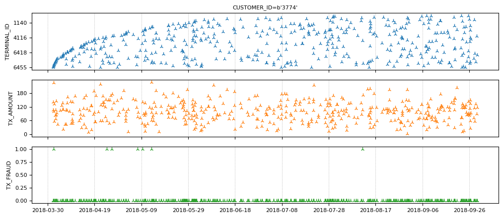
注意该客户的欺诈交易很少。
准备训练数据
孤立的欺诈交易无法被检测到。相反,我们需要连接相关的交易。对于每笔交易,我们计算过去 n 天内同一终端的交易总数和计数。由于我们不知道 n 的正确值,我们使用多个 n 值并为每个值计算一组特征。
# Group the transactions per terminal
transactions_per_terminal = transactions_evset.add_index("TERMINAL_ID")

# Moving statistics per terminal
tmp_features = []
for n in [7, 14, 28]:
    tmp_features.append(
        transactions_per_terminal["TX_AMOUNT"]
        .moving_sum(tp.duration.days(n))
        .rename(f"sum_transactions_{n}_days")
    )

    tmp_features.append(
        transactions_per_terminal.moving_count(tp.duration.days(n)).rename(
            f"count_transactions_{n}_days"
        )
    )

feature_set_1 = tp.glue(*tmp_features)

feature_set_1
| 时间戳 | sum_transactions_7_days | count_transactions_7_days | sum_transactions_14_days | count_transactions_14_days | sum_transactions_28_days | count_transactions_28_days |
|---|---|---|---|---|---|---|
| 2018-04-02 01:00:01+00:00 | 16.07 | 1 | 16.07 | 1 | 16.07 | 1 |
| 2018-04-02 09:49:55+00:00 | 83.9 | 2 | 83.9 | 2 | 83.9 | 2 |
| 2018-04-03 12:14:41+00:00 | 110.7 | 3 | 110.7 | 3 | 110.7 | 3 |
| 2018-04-05 16:47:41+00:00 | 151.2 | 4 | 151.2 | 4 | 151.2 | 4 |
| 2018-04-07 06:05:21+00:00 | 199.6 | 5 | 199.6 | 5 | 199.6 | 5 |
| … | … | … | … | … | … | … |
| 时间戳 | sum_transactions_7_days | count_transactions_7_days | sum_transactions_14_days | count_transactions_14_days | sum_transactions_28_days | count_transactions_28_days |
|---|---|---|---|---|---|---|
| 2018-04-01 16:24:39+00:00 | 70.36 | 1 | 70.36 | 1 | 70.36 | 1 |
| 2018-04-02 11:25:03+00:00 | 87.79 | 2 | 87.79 | 2 | 87.79 | 2 |
| 2018-04-04 08:31:48+00:00 | 211.6 | 3 | 211.6 | 3 | 211.6 | 3 |
| 2018-04-04 14:15:28+00:00 | 315 | 4 | 315 | 4 | 315 | 4 |
| 2018-04-04 20:54:17+00:00 | 446.5 | 5 | 446.5 | 5 | 446.5 | 5 |
| … | … | … | … | … | … | … |
| 时间戳 | sum_transactions_7_days | count_transactions_7_days | sum_transactions_14_days | count_transactions_14_days | sum_transactions_28_days | count_transactions_28_days |
|---|---|---|---|---|---|---|
| 2018-04-01 14:11:55+00:00 | 2.9 | 1 | 2.9 | 1 | 2.9 | 1 |
| 2018-04-02 11:01:07+00:00 | 17.04 | 2 | 17.04 | 2 | 17.04 | 2 |
| 2018-04-03 13:46:58+00:00 | 118.2 | 3 | 118.2 | 3 | 118.2 | 3 |
| 2018-04-04 03:27:11+00:00 | 161.7 | 4 | 161.7 | 4 | 161.7 | 4 |
| 2018-04-05 17:58:10+00:00 | 171.3 | 5 | 171.3 | 5 | 171.3 | 5 |
| … | … | … | … | … | … | … |
| 时间戳 | sum_transactions_7_days | count_transactions_7_days | sum_transactions_14_days | count_transactions_14_days | sum_transactions_28_days | count_transactions_28_days |
|---|---|---|---|---|---|---|
| 2018-04-02 10:37:42+00:00 | 6.31 | 1 | 6.31 | 1 | 6.31 | 1 |
| 2018-04-04 19:14:23+00:00 | 12.26 | 2 | 12.26 | 2 | 12.26 | 2 |
| 2018-04-07 04:01:22+00:00 | 65.12 | 3 | 65.12 | 3 | 65.12 | 3 |
| 2018-04-07 12:18:27+00:00 | 112.4 | 4 | 112.4 | 4 | 112.4 | 4 |
| 2018-04-07 21:11:03+00:00 | 170.4 | 5 | 170.4 | 5 | 170.4 | 5 |
| … | … | … | … | … | … | … |
让我们看看终端“3774”的特征。
feature_set_1.plot(indexes="3774")
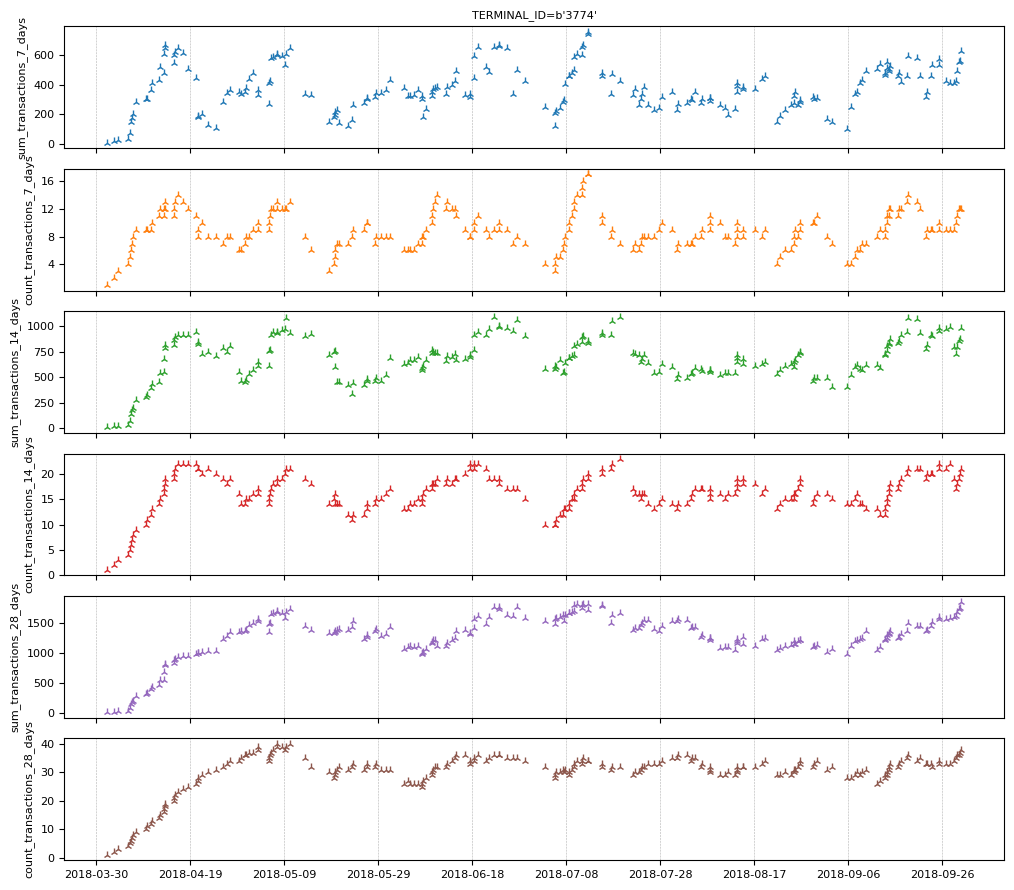
交易的欺诈状态在交易时是未知的(否则就不会有问题)。但是,银行在一周后才知道交易是否为欺诈。我们创建一组特征,指示过去 N 天内欺诈交易的数量和比例。
# Lag the transactions by one week.
lagged_transactions = transactions_per_terminal.lag(tp.duration.weeks(1))

# Moving statistics per customer
tmp_features = []
for n in [7, 14, 28]:
    tmp_features.append(
        lagged_transactions["TX_FRAUD"]
        .moving_sum(tp.duration.days(n), sampling=transactions_per_terminal)
        .rename(f"count_fraud_transactions_{n}_days")
    )

    tmp_features.append(
        lagged_transactions["TX_FRAUD"]
        .cast(tp.float32)
        .simple_moving_average(tp.duration.days(n), sampling=transactions_per_terminal)
        .rename(f"rate_fraud_transactions_{n}_days")
    )

feature_set_2 = tp.glue(*tmp_features)
交易日期和时间可能与欺诈相关。虽然每笔交易都有时间戳,但机器学习模型可能难以直接使用它们。相反,我们从时间戳中提取各种信息日历特征,例如小时、星期几(例如,星期一、星期二)和月份中的哪一天(1-31)。
feature_set_3 = tp.glue(
    transactions_per_terminal.calendar_hour(),
    transactions_per_terminal.calendar_day_of_week(),
)
最后,我们将所有特征和标签组合在一起。
all_data = tp.glue(
    transactions_per_terminal, feature_set_1, feature_set_2, feature_set_3
).drop_index()

print("All the available features:")
all_data.schema.feature_names()
All the available features:

['CUSTOMER_ID',
 'TX_AMOUNT',
 'TX_FRAUD',
 'sum_transactions_7_days',
 'count_transactions_7_days',
 'sum_transactions_14_days',
 'count_transactions_14_days',
 'sum_transactions_28_days',
 'count_transactions_28_days',
 'count_fraud_transactions_7_days',
 'rate_fraud_transactions_7_days',
 'count_fraud_transactions_14_days',
 'rate_fraud_transactions_14_days',
 'count_fraud_transactions_28_days',
 'rate_fraud_transactions_28_days',
 'calendar_hour',
 'calendar_day_of_week',
 'TERMINAL_ID']
我们提取输入特征的名称。
input_feature_names = [k for k in all_data.schema.feature_names() if k.islower()]

print("The model's input features:")
input_feature_names
The model's input features:

['sum_transactions_7_days',
 'count_transactions_7_days',
 'sum_transactions_14_days',
 'count_transactions_14_days',
 'sum_transactions_28_days',
 'count_transactions_28_days',
 'count_fraud_transactions_7_days',
 'rate_fraud_transactions_7_days',
 'count_fraud_transactions_14_days',
 'rate_fraud_transactions_14_days',
 'count_fraud_transactions_28_days',
 'rate_fraud_transactions_28_days',
 'calendar_hour',
 'calendar_day_of_week']
为了使神经网络正常工作,数值输入必须被标准化。一种常见的方法是应用 z 标准化,即从训练数据中估计的平均值和标准差中减去每个值。在预测中,不建议进行此类 z 标准化,因为它会导致未来泄露。具体来说,为了在时间 t 对交易进行分类,我们不能依赖时间 t 之后的数据,因为在提供服务时,当在时间 t 进行预测时,后续数据尚不可用。简而言之,在时间 t,我们只能使用早于或等于时间 t 的数据。
因此,解决方案是按时间应用 z 标准化,这意味着我们使用为该交易计算的过去数据计算出的平均值和标准差来标准化每笔交易。
未来泄露是潜移默化的。幸运的是,Temporian 在此为您提供帮助:唯一可能导致未来泄露的操作符是 EventSet.leak()。如果您不使用 EventSet.leak(),您的预处理保证不会产生未来泄露。
注意:对于高级管道,您也可以通过编程方式检查特征是否不依赖于 EventSet.leak() 操作。
# Cast all values (e.g. ints) to floats.
values = all_data[input_feature_names].cast(tp.float32)

# Apply z-normalization overtime.
normalized_features = (
    values - values.simple_moving_average(math.inf)
) / values.moving_standard_deviation(math.inf)

# Restore the original name of the features.
normalized_features = normalized_features.rename(values.schema.feature_names())

print(normalized_features)
indexes: []
features: [('sum_transactions_7_days', float32), ('count_transactions_7_days', float32), ('sum_transactions_14_days', float32), ('count_transactions_14_days', float32), ('sum_transactions_28_days', float32), ('count_transactions_28_days', float32), ('count_fraud_transactions_7_days', float32), ('rate_fraud_transactions_7_days', float32), ('count_fraud_transactions_14_days', float32), ('rate_fraud_transactions_14_days', float32), ('count_fraud_transactions_28_days', float32), ('rate_fraud_transactions_28_days', float32), ('calendar_hour', float32), ('calendar_day_of_week', float32)]
events:
     (1754155 events):
        timestamps: ['2018-04-01T00:00:31' '2018-04-01T00:02:10' '2018-04-01T00:07:56' ...
     '2018-09-30T23:58:21' '2018-09-30T23:59:52' '2018-09-30T23:59:57']
        'sum_transactions_7_days': [ 0.      1.      1.3636 ... -0.064  -0.2059  0.8428]
        'count_transactions_7_days': [   nan    nan    nan ... 1.0128 0.6892 1.66  ]
        'sum_transactions_14_days': [ 0.      1.      1.3636 ... -0.7811  0.156   1.379 ]
        'count_transactions_14_days': [   nan    nan    nan ... 0.2969 0.2969 2.0532]
        'sum_transactions_28_days': [ 0.      1.      1.3636 ... -0.7154 -0.2989  1.9396]
        'count_transactions_28_days': [    nan     nan     nan ...  0.1172 -0.1958  1.8908]
        'count_fraud_transactions_7_days': [    nan     nan     nan ... -0.1043 -0.1043 -0.1043]
        'rate_fraud_transactions_7_days': [    nan     nan     nan ... -0.1137 -0.1137 -0.1137]
        'count_fraud_transactions_14_days': [    nan     nan     nan ... -0.1133 -0.1133  0.9303]
        'rate_fraud_transactions_14_days': [    nan     nan     nan ... -0.1216 -0.1216  0.5275]
        ...
memory usage: 112.3 MB
/home/gbm/my_venv/lib/python3.11/site-packages/temporian/implementation/numpy/operators/binary/arithmetic.py:100: RuntimeWarning: invalid value encountered in divide
  return evset_1_feature / evset_2_feature
由于早期数据量很少,因此最初的交易将使用不准确的平均值和标准差进行标准化。为了缓解这个问题,我们从训练数据集中删除了前一周的数据。
请注意,前几个值包含 NaN。在 Temporian 中,NaN 表示缺失值,所有操作符都会相应地处理它们。例如,在计算移动平均值时,NaN 值不包含在计算中,也不会生成 NaN 结果。
但是,神经网络无法原生处理 NaN 值。因此,我们将它们替换为零。
normalized_features = normalized_features.fillna(0.0)
最后,我们将特征和标签组合在一起。
normalized_all_data = tp.glue(normalized_features, all_data["TX_FRAUD"])
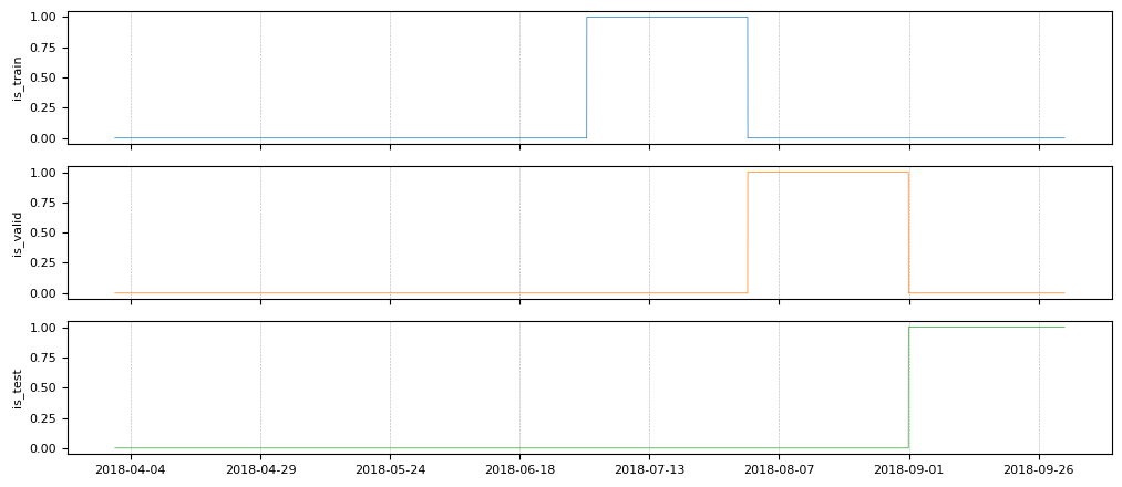
将数据集分割为训练集、验证集和测试集
为了评估我们机器学习模型的质量,我们需要训练集、验证集和测试集。由于系统是动态的(欺诈模式一直在不断出现),因此训练集必须早于验证集,验证集必须早于测试集,这一点很重要。
- 训练: 2018 年 4 月 8 日至 2018 年 7 月 31 日
- 验证: 2018 年 8 月 1 日至 2018 年 8 月 31 日
- 测试: 2018 年 9 月 1 日至 2018 年 9 月 30 日
为了使示例运行得更快,我们将有效缩减训练集的大小为:- 训练: 2018 年 7 月 1 日至 2018 年 7 月 31 日
# begin_train = datetime.datetime(2018, 4, 8).timestamp() # Full training dataset
begin_train = datetime.datetime(2018, 7, 1).timestamp()  # Reduced training dataset
begin_valid = datetime.datetime(2018, 8, 1).timestamp()
begin_test = datetime.datetime(2018, 9, 1).timestamp()

is_train = (normalized_all_data.timestamps() >= begin_train) & (
    normalized_all_data.timestamps() < begin_valid
)
is_valid = (normalized_all_data.timestamps() >= begin_valid) & (
    normalized_all_data.timestamps() < begin_test
)
is_test = normalized_all_data.timestamps() >= begin_test
is_train、is_valid 和 is_test 是随时间变化的布尔特征,它们指示了树折叠的界限。让我们绘制它们。
tp.plot(
    [
        is_train.rename("is_train"),
        is_valid.rename("is_valid"),
        is_test.rename("is_test"),
    ]
)
我们在每个折叠中过滤输入特征和标签。
train_ds_evset = normalized_all_data.filter(is_train)
valid_ds_evset = normalized_all_data.filter(is_valid)
test_ds_evset = normalized_all_data.filter(is_test)

print(f"Training examples: {train_ds_evset.num_events()}")
print(f"Validation examples: {valid_ds_evset.num_events()}")
print(f"Testing examples: {test_ds_evset.num_events()}")
Training examples: 296924
Validation examples: 296579
Testing examples: 288064
在计算完特征之后分割数据集很重要,因为训练集的一些特征是从训练窗口内的交易计算得出的。
创建 TensorFlow 数据集
我们将数据集从 EventSets 转换为 TensorFlow 数据集,因为 Keras 可以原生使用它们。
non_batched_train_ds = tp.to_tensorflow_dataset(train_ds_evset)
non_batched_valid_ds = tp.to_tensorflow_dataset(valid_ds_evset)
non_batched_test_ds = tp.to_tensorflow_dataset(test_ds_evset)
以下处理步骤使用 TensorFlow 数据集进行应用
- 使用
extract_features_and_label将特征和标签分离,以 Keras 所需的格式。 - 数据集被分批,这意味着示例被分组到小批量中。
- 对训练示例进行混洗,以提高小批量训练的质量。
正如我们之前注意到的,数据集在合法交易方面是不平衡的。虽然我们希望在原始分布上评估模型,但神经网络在强烈不平衡的数据集上的训练效果通常不佳。因此,我们使用 rejection_resample 将训练数据集重新采样为 80% 合法 / 20% 欺诈的比例。
def extract_features_and_label(example):
    features = {k: example[k] for k in input_feature_names}
    labels = tf.cast(example["TX_FRAUD"], tf.int32)
    return features, labels


# Target ratio of fraudulent transactions in the training dataset.
target_rate = 0.2

# Number of examples in a mini-batch.
batch_size = 32

train_ds = (
    non_batched_train_ds.shuffle(10000)
    .rejection_resample(
        class_func=lambda x: tf.cast(x["TX_FRAUD"], tf.int32),
        target_dist=[1 - target_rate, target_rate],
        initial_dist=[1 - fraudulent_rate, fraudulent_rate],
    )
    .map(lambda _, x: x)  # Remove the label copy added by "rejection_resample".
    .batch(batch_size)
    .map(extract_features_and_label)
    .prefetch(tf.data.AUTOTUNE)
)

# The test and validation dataset does not need resampling or shuffling.
valid_ds = (
    non_batched_valid_ds.batch(batch_size)
    .map(extract_features_and_label)
    .prefetch(tf.data.AUTOTUNE)
)
test_ds = (
    non_batched_test_ds.batch(batch_size)
    .map(extract_features_and_label)
    .prefetch(tf.data.AUTOTUNE)
)
WARNING:tensorflow:From /home/gbm/my_venv/lib/python3.11/site-packages/tensorflow/python/data/ops/dataset_ops.py:4956: Print (from tensorflow.python.ops.logging_ops) is deprecated and will be removed after 2018-08-20.
Instructions for updating:
Use tf.print instead of tf.Print. Note that tf.print returns a no-output operator that directly prints the output. Outside of defuns or eager mode, this operator will not be executed unless it is directly specified in session.run or used as a control dependency for other operators. This is only a concern in graph mode. Below is an example of how to ensure tf.print executes in graph mode:
我们打印训练数据集的前四个示例。这是一种识别上方可能出现的某些错误的方法。
for features, labels in train_ds.take(1):
    print("features")
    for feature_name, feature_value in features.items():
        print(f"\t{feature_name}: {feature_value[:4]}")
    print(f"labels: {labels[:4]}")
features
    sum_transactions_7_days: [-0.9417254 -1.1157728 -0.5594417  0.7264878]
    count_transactions_7_days: [-0.23363686 -0.8702531  -0.23328805  0.7198456 ]
    sum_transactions_14_days: [-0.9084115  2.8127224  0.7297886  0.0666021]
    count_transactions_14_days: [-0.54289246  2.4122045   0.1963075   0.3798441 ]
    sum_transactions_28_days: [-0.44202712  2.3494742   0.20992276  0.97425723]
    count_transactions_28_days: [0.02585898 1.8197156  0.12127225 0.9692807 ]
    count_fraud_transactions_7_days: [ 8.007475   -0.09783722  1.9282814  -0.09780706]
    rate_fraud_transactions_7_days: [14.308702   -0.10952345  1.6929103  -0.10949575]
    count_fraud_transactions_14_days: [12.411182  -0.1045466  1.0330476 -0.1045142]
    rate_fraud_transactions_14_days: [15.742149   -0.11567765  1.0170861  -0.11565071]
    count_fraud_transactions_28_days: [ 7.420907   -0.11298086  0.572011   -0.11293571]
    rate_fraud_transactions_28_days: [10.065552   -0.12640427  0.5862939  -0.12637936]
    calendar_hour: [-0.68766755  0.6972711  -1.6792761   0.49967623]
    calendar_day_of_week: [1.492013  1.4789637 1.4978485 1.4818214]
labels: [1 0 0 0]

Proportion of examples rejected by sampler is high: [0.991630733][0.991630733 0.00836927164][0 1]
Proportion of examples rejected by sampler is high: [0.991630733][0.991630733 0.00836927164][0 1]
Proportion of examples rejected by sampler is high: [0.991630733][0.991630733 0.00836927164][0 1]
Proportion of examples rejected by sampler is high: [0.991630733][0.991630733 0.00836927164][0 1]
Proportion of examples rejected by sampler is high: [0.991630733][0.991630733 0.00836927164][0 1]
Proportion of examples rejected by sampler is high: [0.991630733][0.991630733 0.00836927164][0 1]
Proportion of examples rejected by sampler is high: [0.991630733][0.991630733 0.00836927164][0 1]
Proportion of examples rejected by sampler is high: [0.991630733][0.991630733 0.00836927164][0 1]
Proportion of examples rejected by sampler is high: [0.991630733][0.991630733 0.00836927164][0 1]
Proportion of examples rejected by sampler is high: [0.991630733][0.991630733 0.00836927164][0 1]
训练模型
原始数据集是交易数据,但处理后的数据是表格数据,仅包含标准化的数值。因此,我们训练一个前馈神经网络。
inputs = [keras.Input(shape=(1,), name=name) for name in input_feature_names]
x = keras.layers.concatenate(inputs)
x = keras.layers.Dense(32, activation="sigmoid")(x)
x = keras.layers.Dense(16, activation="sigmoid")(x)
x = keras.layers.Dense(1, activation="sigmoid")(x)
model = keras.Model(inputs=inputs, outputs=x)
我们的目标是区分欺诈交易和合法交易,因此我们使用二元分类目标。由于数据集不平衡,准确率不是一个有用的指标。相反,我们使用 曲线下面积 (AUC) 来评估模型。
model.compile(
    optimizer=keras.optimizers.Adam(0.01),
    loss=keras.losses.BinaryCrossentropy(),
    metrics=[keras.metrics.Accuracy(), keras.metrics.AUC()],
)
model.fit(train_ds, validation_data=valid_ds)
      5/Unknown  1s 15ms/step - accuracy: 0.0000e+00 - auc: 0.4480 - loss: 0.7678

Proportion of examples rejected by sampler is high: [0.991630733][0.991630733 0.00836927164][0 1]
Proportion of examples rejected by sampler is high: [0.991630733][0.991630733 0.00836927164][0 1]
Proportion of examples rejected by sampler is high: [0.991630733][0.991630733 0.00836927164][0 1]
Proportion of examples rejected by sampler is high: [0.991630733][0.991630733 0.00836927164][0 1]
Proportion of examples rejected by sampler is high: [0.991630733][0.991630733 0.00836927164][0 1]
Proportion of examples rejected by sampler is high: [0.991630733][0.991630733 0.00836927164][0 1]
Proportion of examples rejected by sampler is high: [0.991630733][0.991630733 0.00836927164][0 1]
Proportion of examples rejected by sampler is high: [0.991630733][0.991630733 0.00836927164][0 1]
Proportion of examples rejected by sampler is high: [0.991630733][0.991630733 0.00836927164][0 1]
Proportion of examples rejected by sampler is high: [0.991630733][0.991630733 0.00836927164][0 1]

    433/Unknown  23s 51ms/step - accuracy: 0.0000e+00 - auc: 0.8060 - loss: 0.3632

/usr/lib/python3.11/contextlib.py:155: UserWarning: Your input ran out of data; interrupting training. Make sure that your dataset or generator can generate at least `steps_per_epoch * epochs` batches. You may need to use the `.repeat()` function when building your dataset.
  self.gen.throw(typ, value, traceback)

 433/433 ━━━━━━━━━━━━━━━━━━━━ 30s 67ms/step - accuracy: 0.0000e+00 - auc: 0.8060 - loss: 0.3631 - val_accuracy: 0.0000e+00 - val_auc: 0.8252 - val_loss: 0.2133

<keras.src.callbacks.history.History at 0x7f8f74f0d750>
我们在测试数据集上评估模型。
model.evaluate(test_ds)
 9002/9002 ━━━━━━━━━━━━━━━━━━━━ 7s 811us/step - accuracy: 0.0000e+00 - auc: 0.8357 - loss: 0.2161

[0.2171599417924881, 0.0, 0.8266682028770447]
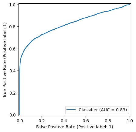
AUC 约为 83%,我们的简单欺诈检测器显示出令人鼓舞的结果。
绘制 ROC 曲线是理解和选择模型操作点的绝佳方法,即用于区分欺诈和合法交易的模型输出阈值。
计算测试预测
predictions = model.predict(test_ds)
predictions = np.nan_to_num(predictions, nan=0)
9002/9002 ━━━━━━━━━━━━━━━━━━━━ 10s 1ms/step
从测试集中提取标签
labels = np.concatenate([label for _, label in test_ds])
最后,我们绘制 ROC 曲线。
_ = RocCurveDisplay.from_predictions(labels, predictions)
Keras 模型已准备好用于具有未知欺诈状态的交易,即服务。我们将模型保存到磁盘以备将来使用。
注意: 模型不包含在 Pandas 和 Temporian 中完成的数据准备和预处理步骤。它们必须手动应用于输入到模型中的数据。虽然此处未演示,但 Temporian 预处理也可以使用 tp.save 保存到磁盘。
model.save("fraud_detection_model.keras")
模型稍后可以使用以下方式重新加载
loaded_model = keras.saving.load_model("fraud_detection_model.keras")

# Generate predictions with the loaded model on 5 test examples.
loaded_model.predict(test_ds.rebatch(5).take(1))
 1/1 ━━━━━━━━━━━━━━━━━━━━ 0s 71ms/step

/usr/lib/python3.11/contextlib.py:155: UserWarning: Your input ran out of data; interrupting training. Make sure that your dataset or generator can generate at least `steps_per_epoch * epochs` batches. You may need to use the `.repeat()` function when building your dataset.
  self.gen.throw(typ, value, traceback)

array([[0.08197185],
       [0.16517264],
       [0.13180313],
       [0.10209075],
       [0.14283912]], dtype=float32)
结论
我们训练了一个前馈神经网络来识别欺诈交易。为了将它们输入模型,使用 Temporian 对交易进行了预处理并转换为表格数据集。现在,向读者提出一个问题:还可以做些什么来进一步提高模型的性能?
以下是一些想法
- 在整个数据集上训练模型,而不是在单个月份的数据上训练。
- 训练模型更多轮次,并使用早停法来确保模型已完全训练而不过拟合。
- 通过增加层数使前馈网络更强大,同时确保模型得到正则化。
- 计算额外的预处理特征。例如,除了按终端聚合交易外,还按客户聚合交易。
- 使用 Keras Tuner 对模型进行超参数调优。请注意,预处理的参数(例如,聚合的天数)也是可以调优的超参数。