► 代码示例 / 时间序列 / 用于动作识别的脑电图信号分类

用于动作识别的脑电图信号分类

作者： Suvaditya Mukherjee
创建日期 2022/11/03
最后修改日期 2022/11/05
描述： 训练卷积模型以分类由特定刺激引起的脑电图信号。

ⓘ 此示例使用 Keras 3

简介

以下示例探讨了我们如何构建一个基于卷积的神经网络，以对受试者暴露于不同刺激时捕获的脑电图信号进行分类。我们从头开始训练模型，因为这种信号分类模型在预训练格式中相当稀缺。我们使用的数据来自加州大学伯克利分校生物传感实验室，数据同时从 15 名受试者处收集。我们的流程如下：

加载加州大学伯克利分校生物传感同步脑电波数据集
可视化数据中的随机样本
预处理、整理和缩放数据，最终制作一个 tf.data.Dataset
准备类别权重以解决主要的不平衡问题
创建一个基于 Conv1D 和 Dense 的模型来执行分类
定义回调和超参数
训练模型
绘制来自 History 的指标并执行评估

此示例需要以下外部依赖项 (Gdown, Scikit-learn, Pandas, Numpy, Matplotlib)。您可以通过以下命令安装它。

Gdown 是一个外部软件包，用于从 Google Drive 下载大型文件。要了解更多信息，您可以参考其 PyPi 页面

设置和数据下载

首先，让我们安装我们的依赖项

!pip install gdown -q
!pip install sklearn -q
!pip install pandas -q
!pip install numpy -q
!pip install matplotlib -q

接下来，让我们下载我们的数据集。gdown 软件包可以轻松地从 Google Drive 下载数据

!gdown 1V5B7Bt6aJm0UHbR7cRKBEK8jx7lYPVuX
!# gdown will download eeg-data.csv onto the local drive for use. Total size of
!# eeg-data.csv is 105.7 MB

import pandas as pd
import matplotlib.pyplot as plt
import json
import numpy as np
import keras
from keras import layers
import tensorflow as tf
from sklearn import preprocessing, model_selection
import random

QUALITY_THRESHOLD = 128
BATCH_SIZE = 64
SHUFFLE_BUFFER_SIZE = BATCH_SIZE * 2

Downloading...
From (uriginal): https://drive.google.com/uc?id=1V5B7Bt6aJm0UHbR7cRKBEK8jx7lYPVuX
From (redirected): https://drive.google.com/uc?id=1V5B7Bt6aJm0UHbR7cRKBEK8jx7lYPVuX&confirm=t&uuid=4d50d1e7-44b5-4984-aa04-cb4e08803cb8
To: /home/fchollet/keras-io/scripts/tmp_3333846/eeg-data.csv
100%|█████████████████████████████████████████| 106M/106M [00:00<00:00, 259MB/s]

从 `eeg-data.csv` 读取数据

我们使用 Pandas 库读取 eeg-data.csv 文件，并使用 .head() 命令显示前 5 行

eeg = pd.read_csv("eeg-data.csv")

我们从数据集中删除未标记的样本，因为它们对模型没有贡献。我们还在训练数据准备不需要的列上执行 .drop() 操作

unlabeled_eeg = eeg[eeg["label"] == "unlabeled"]
eeg = eeg.loc[eeg["label"] != "unlabeled"]
eeg = eeg.loc[eeg["label"] != "everyone paired"]

eeg.drop(
    [
        "indra_time",
        "Unnamed: 0",
        "browser_latency",
        "reading_time",
        "attention_esense",
        "meditation_esense",
        "updatedAt",
        "createdAt",
    ],
    axis=1,
    inplace=True,
)

eeg.reset_index(drop=True, inplace=True)
eeg.head()

	id	eeg_power	raw_values	label
0	7	[56887.0, 45471.0, 20074.0, 5359.0, 22594.0, 7...	[99.0, 96.0, 91.0, 89.0, 91.0, 89.0, 87.0, 93....	blinkInstruction
1	5	[11626.0, 60301.0, 5805.0, 15729.0, 4448.0, 33...	[23.0, 40.0, 64.0, 89.0, 86.0, 33.0, -14.0, -1...	blinkInstruction
2	1	[15777.0, 33461.0, 21385.0, 44193.0, 11741.0, ...	[41.0, 26.0, 16.0, 20.0, 34.0, 51.0, 56.0, 55....	blinkInstruction
3	13	[311822.0, 44739.0, 19000.0, 19100.0, 2650.0, ...	[208.0, 198.0, 122.0, 84.0, 161.0, 249.0, 216....	blinkInstruction
4	4	[687393.0, 10289.0, 2942.0, 9874.0, 1059.0, 29...	[129.0, 133.0, 114.0, 105.0, 101.0, 109.0, 99....	blinkInstruction

在数据中，记录的样本根据传感器校准的良好程度（0 为最佳，200 为最差）给出 0 到 128 的分数。我们根据 128 的任意截止限制过滤值。

def convert_string_data_to_values(value_string):
    str_list = json.loads(value_string)
    return str_list


eeg["raw_values"] = eeg["raw_values"].apply(convert_string_data_to_values)

eeg = eeg.loc[eeg["signal_quality"] < QUALITY_THRESHOLD]
eeg.head()

	id	eeg_power	raw_values	label
0	7	[56887.0, 45471.0, 20074.0, 5359.0, 22594.0, 7...	[99.0, 96.0, 91.0, 89.0, 91.0, 89.0, 87.0, 93....	blinkInstruction
1	5	[11626.0, 60301.0, 5805.0, 15729.0, 4448.0, 33...	[23.0, 40.0, 64.0, 89.0, 86.0, 33.0, -14.0, -1...	blinkInstruction
2	1	[15777.0, 33461.0, 21385.0, 44193.0, 11741.0, ...	[41.0, 26.0, 16.0, 20.0, 34.0, 51.0, 56.0, 55....	blinkInstruction
3	13	[311822.0, 44739.0, 19000.0, 19100.0, 2650.0, ...	[208.0, 198.0, 122.0, 84.0, 161.0, 249.0, 216....	blinkInstruction
4	4	[687393.0, 10289.0, 2942.0, 9874.0, 1059.0, 29...	[129.0, 133.0, 114.0, 105.0, 101.0, 109.0, 99....	blinkInstruction

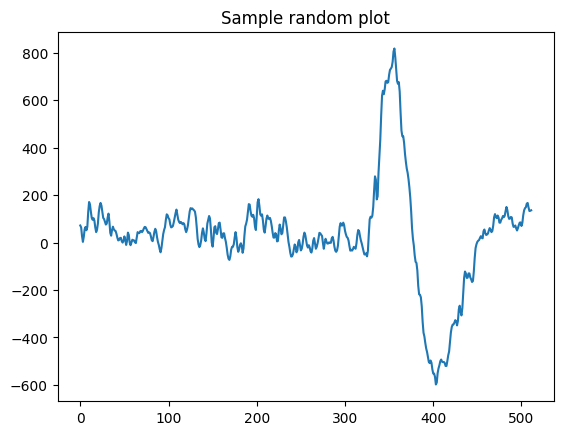
可视化数据中的一个随机样本

我们可视化数据中的一个样本，以了解刺激引起的信号的外观

def view_eeg_plot(idx):
    data = eeg.loc[idx, "raw_values"]
    plt.plot(data)
    plt.title(f"Sample random plot")
    plt.show()


view_eeg_plot(7)

png

预处理和整理数据

数据中总共有 67 个不同的标签，其中有编号的子标签。我们根据它们的编号将它们整理在单个标签下，并在数据本身中替换它们。在此过程之后，我们执行简单的标签编码以将其转换为整数格式。

print("Before replacing labels")
print(eeg["label"].unique(), "\n")
print(len(eeg["label"].unique()), "\n")


eeg.replace(
    {
        "label": {
            "blink1": "blink",
            "blink2": "blink",
            "blink3": "blink",
            "blink4": "blink",
            "blink5": "blink",
            "math1": "math",
            "math2": "math",
            "math3": "math",
            "math4": "math",
            "math5": "math",
            "math6": "math",
            "math7": "math",
            "math8": "math",
            "math9": "math",
            "math10": "math",
            "math11": "math",
            "math12": "math",
            "thinkOfItems-ver1": "thinkOfItems",
            "thinkOfItems-ver2": "thinkOfItems",
            "video-ver1": "video",
            "video-ver2": "video",
            "thinkOfItemsInstruction-ver1": "thinkOfItemsInstruction",
            "thinkOfItemsInstruction-ver2": "thinkOfItemsInstruction",
            "colorRound1-1": "colorRound1",
            "colorRound1-2": "colorRound1",
            "colorRound1-3": "colorRound1",
            "colorRound1-4": "colorRound1",
            "colorRound1-5": "colorRound1",
            "colorRound1-6": "colorRound1",
            "colorRound2-1": "colorRound2",
            "colorRound2-2": "colorRound2",
            "colorRound2-3": "colorRound2",
            "colorRound2-4": "colorRound2",
            "colorRound2-5": "colorRound2",
            "colorRound2-6": "colorRound2",
            "colorRound3-1": "colorRound3",
            "colorRound3-2": "colorRound3",
            "colorRound3-3": "colorRound3",
            "colorRound3-4": "colorRound3",
            "colorRound3-5": "colorRound3",
            "colorRound3-6": "colorRound3",
            "colorRound4-1": "colorRound4",
            "colorRound4-2": "colorRound4",
            "colorRound4-3": "colorRound4",
            "colorRound4-4": "colorRound4",
            "colorRound4-5": "colorRound4",
            "colorRound4-6": "colorRound4",
            "colorRound5-1": "colorRound5",
            "colorRound5-2": "colorRound5",
            "colorRound5-3": "colorRound5",
            "colorRound5-4": "colorRound5",
            "colorRound5-5": "colorRound5",
            "colorRound5-6": "colorRound5",
            "colorInstruction1": "colorInstruction",
            "colorInstruction2": "colorInstruction",
            "readyRound1": "readyRound",
            "readyRound2": "readyRound",
            "readyRound3": "readyRound",
            "readyRound4": "readyRound",
            "readyRound5": "readyRound",
            "colorRound1": "colorRound",
            "colorRound2": "colorRound",
            "colorRound3": "colorRound",
            "colorRound4": "colorRound",
            "colorRound5": "colorRound",
        }
    },
    inplace=True,
)

print("After replacing labels")
print(eeg["label"].unique())
print(len(eeg["label"].unique()))

le = preprocessing.LabelEncoder()  # Generates a look-up table
le.fit(eeg["label"])
eeg["label"] = le.transform(eeg["label"])

Before replacing labels
['blinkInstruction' 'blink1' 'blink2' 'blink3' 'blink4' 'blink5'
 'relaxInstruction' 'relax' 'mathInstruction' 'math1' 'math2' 'math3'
 'math4' 'math5' 'math6' 'math7' 'math8' 'math9' 'math10' 'math11'
 'math12' 'musicInstruction' 'music' 'videoInstruction' 'video-ver1'
 'thinkOfItemsInstruction-ver1' 'thinkOfItems-ver1' 'colorInstruction1'
 'colorInstruction2' 'readyRound1' 'colorRound1-1' 'colorRound1-2'
 'colorRound1-3' 'colorRound1-4' 'colorRound1-5' 'colorRound1-6'
 'readyRound2' 'colorRound2-1' 'colorRound2-2' 'colorRound2-3'
 'colorRound2-4' 'colorRound2-5' 'colorRound2-6' 'readyRound3'
 'colorRound3-1' 'colorRound3-2' 'colorRound3-3' 'colorRound3-4'
 'colorRound3-5' 'colorRound3-6' 'readyRound4' 'colorRound4-1'
 'colorRound4-2' 'colorRound4-3' 'colorRound4-4' 'colorRound4-5'
 'colorRound4-6' 'readyRound5' 'colorRound5-1' 'colorRound5-2'
 'colorRound5-3' 'colorRound5-4' 'colorRound5-5' 'colorRound5-6'
 'video-ver2' 'thinkOfItemsInstruction-ver2' 'thinkOfItems-ver2']

After replacing labels
['blinkInstruction' 'blink' 'relaxInstruction' 'relax' 'mathInstruction'
 'math' 'musicInstruction' 'music' 'videoInstruction' 'video'
 'thinkOfItemsInstruction' 'thinkOfItems' 'colorInstruction' 'readyRound'
 'colorRound1' 'colorRound2' 'colorRound3' 'colorRound4' 'colorRound5']
19

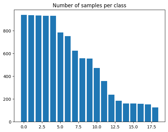
我们提取数据中存在的唯一类别的数量

num_classes = len(eeg["label"].unique())
print(num_classes)

我们现在使用条形图可视化每个类别中存在的样本数量。

plt.bar(range(num_classes), eeg["label"].value_counts())
plt.title("Number of samples per class")
plt.show()

png

缩放和拆分数据

我们执行简单的 Min-Max 缩放以将值范围控制在 0 到 1 之间。我们不使用标准缩放，因为数据不服从高斯分布。

scaler = preprocessing.MinMaxScaler()
series_list = [
    scaler.fit_transform(np.asarray(i).reshape(-1, 1)) for i in eeg["raw_values"]
]

labels_list = [i for i in eeg["label"]]

我们现在创建一个具有 15% 留出集的训练-测试拆分。在此之后，我们重塑数据以创建长度为 512 的序列。我们还将标签从当前标签编码形式转换为 one-hot 编码，以便可以使用几种不同的 keras.metrics 函数。

x_train, x_test, y_train, y_test = model_selection.train_test_split(
    series_list, labels_list, test_size=0.15, random_state=42, shuffle=True
)

print(
    f"Length of x_train : {len(x_train)}\nLength of x_test : {len(x_test)}\nLength of y_train : {len(y_train)}\nLength of y_test : {len(y_test)}"
)

x_train = np.asarray(x_train).astype(np.float32).reshape(-1, 512, 1)
y_train = np.asarray(y_train).astype(np.float32).reshape(-1, 1)
y_train = keras.utils.to_categorical(y_train)

x_test = np.asarray(x_test).astype(np.float32).reshape(-1, 512, 1)
y_test = np.asarray(y_test).astype(np.float32).reshape(-1, 1)
y_test = keras.utils.to_categorical(y_test)

Length of x_train : 8460
Length of x_test : 1494
Length of y_train : 8460
Length of y_test : 1494

准备 `tf.data.Dataset`

我们现在从此数据创建一个 tf.data.Dataset，以准备用于训练。我们还对数据进行洗牌和批处理，以便稍后使用。

train_dataset = tf.data.Dataset.from_tensor_slices((x_train, y_train))
test_dataset = tf.data.Dataset.from_tensor_slices((x_test, y_test))

train_dataset = train_dataset.shuffle(SHUFFLE_BUFFER_SIZE).batch(BATCH_SIZE)
test_dataset = test_dataset.batch(BATCH_SIZE)

使用朴素方法制作类别权重

正如我们从每个类别的样本数量图中看到的那样，数据集是不平衡的。因此，我们计算每个类别的权重，以确保模型以公平的方式训练，而不会因为样本数量较多而偏向任何特定类别。

我们使用一种朴素的方法来计算这些权重，找到每个类别的反比例，并将其用作权重。

vals_dict = {}
for i in eeg["label"]:
    if i in vals_dict.keys():
        vals_dict[i] += 1
    else:
        vals_dict[i] = 1
total = sum(vals_dict.values())

# Formula used - Naive method where
# weight = 1 - (no. of samples present / total no. of samples)
# So more the samples, lower the weight

weight_dict = {k: (1 - (v / total)) for k, v in vals_dict.items()}
print(weight_dict)

{1: 0.9872413100261201, 0: 0.975989551938919, 14: 0.9841269841269842, 13: 0.9061683745228049, 9: 0.9838255977496484, 8: 0.9059674502712477, 11: 0.9847297568816556, 10: 0.9063692987743621, 18: 0.9838255977496484, 17: 0.9057665260196905, 16: 0.9373116335141651, 15: 0.9065702230259193, 2: 0.9211372312638135, 12: 0.9525818766325096, 3: 0.9245529435402853, 4: 0.943841671689773, 5: 0.9641350210970464, 6: 0.981514968856741, 7: 0.9443439823186659}

定义一个简单的函数来绘制 `keras.callbacks.History` 中存在的所有指标

对象

def plot_history_metrics(history: keras.callbacks.History):
    total_plots = len(history.history)
    cols = total_plots // 2

    rows = total_plots // cols

    if total_plots % cols != 0:
        rows += 1

    pos = range(1, total_plots + 1)
    plt.figure(figsize=(15, 10))
    for i, (key, value) in enumerate(history.history.items()):
        plt.subplot(rows, cols, pos[i])
        plt.plot(range(len(value)), value)
        plt.title(str(key))
    plt.show()

定义生成卷积模型的函数

def create_model():
    input_layer = keras.Input(shape=(512, 1))

    x = layers.Conv1D(
        filters=32, kernel_size=3, strides=2, activation="relu", padding="same"
    )(input_layer)
    x = layers.BatchNormalization()(x)

    x = layers.Conv1D(
        filters=64, kernel_size=3, strides=2, activation="relu", padding="same"
    )(x)
    x = layers.BatchNormalization()(x)

    x = layers.Conv1D(
        filters=128, kernel_size=5, strides=2, activation="relu", padding="same"
    )(x)
    x = layers.BatchNormalization()(x)

    x = layers.Conv1D(
        filters=256, kernel_size=5, strides=2, activation="relu", padding="same"
    )(x)
    x = layers.BatchNormalization()(x)

    x = layers.Conv1D(
        filters=512, kernel_size=7, strides=2, activation="relu", padding="same"
    )(x)
    x = layers.BatchNormalization()(x)

    x = layers.Conv1D(
        filters=1024,
        kernel_size=7,
        strides=2,
        activation="relu",
        padding="same",
    )(x)
    x = layers.BatchNormalization()(x)

    x = layers.Dropout(0.2)(x)

    x = layers.Flatten()(x)

    x = layers.Dense(4096, activation="relu")(x)
    x = layers.Dropout(0.2)(x)

    x = layers.Dense(
        2048, activation="relu", kernel_regularizer=keras.regularizers.L2()
    )(x)
    x = layers.Dropout(0.2)(x)

    x = layers.Dense(
        1024, activation="relu", kernel_regularizer=keras.regularizers.L2()
    )(x)
    x = layers.Dropout(0.2)(x)
    x = layers.Dense(
        128, activation="relu", kernel_regularizer=keras.regularizers.L2()
    )(x)
    output_layer = layers.Dense(num_classes, activation="softmax")(x)

    return keras.Model(inputs=input_layer, outputs=output_layer)

获取模型摘要

conv_model = create_model()
conv_model.summary()

Model: "functional_1"

┏━━━━━━━━━━━━━━━━━━━━━━━━━━━━━━━━━┳━━━━━━━━━━━━━━━━━━━━━━━━━━━┳━━━━━━━━━━━━┓
┃ Layer (type)                    ┃ Output Shape              ┃    Param # ┃
┡━━━━━━━━━━━━━━━━━━━━━━━━━━━━━━━━━╇━━━━━━━━━━━━━━━━━━━━━━━━━━━╇━━━━━━━━━━━━┩
│ input_layer (InputLayer)        │ (None, 512, 1)            │          0 │
├─────────────────────────────────┼───────────────────────────┼────────────┤
│ conv1d (Conv1D)                 │ (None, 256, 32)           │        128 │
├─────────────────────────────────┼───────────────────────────┼────────────┤
│ batch_normalization             │ (None, 256, 32)           │        128 │
│ (BatchNormalization)            │                           │            │
├─────────────────────────────────┼───────────────────────────┼────────────┤
│ conv1d_1 (Conv1D)               │ (None, 128, 64)           │      6,208 │
├─────────────────────────────────┼───────────────────────────┼────────────┤
│ batch_normalization_1           │ (None, 128, 64)           │        256 │
│ (BatchNormalization)            │                           │            │
├─────────────────────────────────┼───────────────────────────┼────────────┤
│ conv1d_2 (Conv1D)               │ (None, 64, 128)           │     41,088 │
├─────────────────────────────────┼───────────────────────────┼────────────┤
│ batch_normalization_2           │ (None, 64, 128)           │        512 │
│ (BatchNormalization)            │                           │            │
├─────────────────────────────────┼───────────────────────────┼────────────┤
│ conv1d_3 (Conv1D)               │ (None, 32, 256)           │    164,096 │
├─────────────────────────────────┼───────────────────────────┼────────────┤
│ batch_normalization_3           │ (None, 32, 256)           │      1,024 │
│ (BatchNormalization)            │                           │            │
├─────────────────────────────────┼───────────────────────────┼────────────┤
│ conv1d_4 (Conv1D)               │ (None, 16, 512)           │    918,016 │
├─────────────────────────────────┼───────────────────────────┼────────────┤
│ batch_normalization_4           │ (None, 16, 512)           │      2,048 │
│ (BatchNormalization)            │                           │            │
├─────────────────────────────────┼───────────────────────────┼────────────┤
│ conv1d_5 (Conv1D)               │ (None, 8, 1024)           │  3,671,040 │
├─────────────────────────────────┼───────────────────────────┼────────────┤
│ batch_normalization_5           │ (None, 8, 1024)           │      4,096 │
│ (BatchNormalization)            │                           │            │
├─────────────────────────────────┼───────────────────────────┼────────────┤
│ dropout (Dropout)               │ (None, 8, 1024)           │          0 │
├─────────────────────────────────┼───────────────────────────┼────────────┤
│ flatten (Flatten)               │ (None, 8192)              │          0 │
├─────────────────────────────────┼───────────────────────────┼────────────┤
│ dense (Dense)                   │ (None, 4096)              │ 33,558,528 │
├─────────────────────────────────┼───────────────────────────┼────────────┤
│ dropout_1 (Dropout)             │ (None, 4096)              │          0 │
├─────────────────────────────────┼───────────────────────────┼────────────┤
│ dense_1 (Dense)                 │ (None, 2048)              │  8,390,656 │
├─────────────────────────────────┼───────────────────────────┼────────────┤
│ dropout_2 (Dropout)             │ (None, 2048)              │          0 │
├─────────────────────────────────┼───────────────────────────┼────────────┤
│ dense_2 (Dense)                 │ (None, 1024)              │  2,098,176 │
├─────────────────────────────────┼───────────────────────────┼────────────┤
│ dropout_3 (Dropout)             │ (None, 1024)              │          0 │
├─────────────────────────────────┼───────────────────────────┼────────────┤
│ dense_3 (Dense)                 │ (None, 128)               │    131,200 │
├─────────────────────────────────┼───────────────────────────┼────────────┤
│ dense_4 (Dense)                 │ (None, 19)                │      2,451 │
└─────────────────────────────────┴───────────────────────────┴────────────┘

 Total params: 48,989,651 (186.88 MB)

 Trainable params: 48,985,619 (186.87 MB)

 Non-trainable params: 4,032 (15.75 KB)

定义回调、优化器、损失和指标

在进行了广泛的实验后，我们将 epoch 数设置为 30。结果表明，这是最佳数量，也进行了提前停止分析。我们定义了一个模型检查点回调，以确保我们只获得最佳模型权重。我们还定义了 ReduceLROnPlateau，因为在实验过程中发现了几种损失在某个点之后停滞不前的情况。另一方面，直接 LRScheduler 被发现衰减过于激进。

epochs = 30

callbacks = [
    keras.callbacks.ModelCheckpoint(
        "best_model.keras", save_best_only=True, monitor="loss"
    ),
    keras.callbacks.ReduceLROnPlateau(
        monitor="val_top_k_categorical_accuracy",
        factor=0.2,
        patience=2,
        min_lr=0.000001,
    ),
]

optimizer = keras.optimizers.Adam(amsgrad=True, learning_rate=0.001)
loss = keras.losses.CategoricalCrossentropy()

编译模型并调用 `model.fit()`

我们使用 Adam 优化器，因为它通常被认为是初步训练的最佳选择，并且被发现是最佳优化器。我们使用 CategoricalCrossentropy 作为损失，因为我们的标签采用 one-hot 编码形式。

我们定义了 TopKCategoricalAccuracy(k=3)、AUC、Precision 和 Recall 指标，以进一步帮助更好地理解模型。

conv_model.compile(
    optimizer=optimizer,
    loss=loss,
    metrics=[
        keras.metrics.TopKCategoricalAccuracy(k=3),
        keras.metrics.AUC(),
        keras.metrics.Precision(),
        keras.metrics.Recall(),
    ],
)

conv_model_history = conv_model.fit(
    train_dataset,
    epochs=epochs,
    callbacks=callbacks,
    validation_data=test_dataset,
    class_weight=weight_dict,
)

Epoch 1/30
   8/133 ━[37m━━━━━━━━━━━━━━━━━━━  1s 16ms/step - auc: 0.5550 - loss: 45.5990 - precision: 0.0183 - recall: 0.0049 - top_k_categorical_accuracy: 0.2154

WARNING: All log messages before absl::InitializeLog() is called are written to STDERR
I0000 00:00:1699421521.552287    4412 device_compiler.h:186] Compiled cluster using XLA!  This line is logged at most once for the lifetime of the process.
W0000 00:00:1699421521.578522    4412 graph_launch.cc:671] Fallback to op-by-op mode because memset node breaks graph update

 133/133 ━━━━━━━━━━━━━━━━━━━━ 0s 134ms/step - auc: 0.6119 - loss: 24.8582 - precision: 0.0465 - recall: 0.0022 - top_k_categorical_accuracy: 0.2479

W0000 00:00:1699421539.207966    4409 graph_launch.cc:671] Fallback to op-by-op mode because memset node breaks graph update
W0000 00:00:1699421541.374400    4408 graph_launch.cc:671] Fallback to op-by-op mode because memset node breaks graph update
W0000 00:00:1699421542.991471    4406 graph_launch.cc:671] Fallback to op-by-op mode because memset node breaks graph update

 133/133 ━━━━━━━━━━━━━━━━━━━━ 44s 180ms/step - auc: 0.6122 - loss: 24.7734 - precision: 0.0466 - recall: 0.0022 - top_k_categorical_accuracy: 0.2481 - val_auc: 0.6470 - val_loss: 4.1950 - val_precision: 0.0000e+00 - val_recall: 0.0000e+00 - val_top_k_categorical_accuracy: 0.2610 - learning_rate: 0.0010
Epoch 2/30
 133/133 ━━━━━━━━━━━━━━━━━━━━ 8s 63ms/step - auc: 0.6958 - loss: 3.5651 - precision: 0.0000e+00 - recall: 0.0000e+00 - top_k_categorical_accuracy: 0.3162 - val_auc: 0.6364 - val_loss: 3.3169 - val_precision: 0.0000e+00 - val_recall: 0.0000e+00 - val_top_k_categorical_accuracy: 0.2436 - learning_rate: 0.0010
Epoch 3/30
 133/133 ━━━━━━━━━━━━━━━━━━━━ 8s 63ms/step - auc: 0.7068 - loss: 2.8805 - precision: 0.1910 - recall: 1.2846e-04 - top_k_categorical_accuracy: 0.3220 - val_auc: 0.6313 - val_loss: 3.0662 - val_precision: 0.0000e+00 - val_recall: 0.0000e+00 - val_top_k_categorical_accuracy: 0.2503 - learning_rate: 0.0010
Epoch 4/30
 133/133 ━━━━━━━━━━━━━━━━━━━━ 8s 63ms/step - auc: 0.7370 - loss: 2.6265 - precision: 0.0719 - recall: 2.8215e-04 - top_k_categorical_accuracy: 0.3572 - val_auc: 0.5952 - val_loss: 3.1744 - val_precision: 0.0000e+00 - val_recall: 0.0000e+00 - val_top_k_categorical_accuracy: 0.2282 - learning_rate: 2.0000e-04
Epoch 5/30
 133/133 ━━━━━━━━━━━━━━━━━━━━ 9s 65ms/step - auc: 0.7703 - loss: 2.4886 - precision: 0.3738 - recall: 0.0022 - top_k_categorical_accuracy: 0.4029 - val_auc: 0.6320 - val_loss: 3.3036 - val_precision: 0.0000e+00 - val_recall: 0.0000e+00 - val_top_k_categorical_accuracy: 0.2564 - learning_rate: 2.0000e-04
Epoch 6/30
 133/133 ━━━━━━━━━━━━━━━━━━━━ 9s 66ms/step - auc: 0.8187 - loss: 2.3009 - precision: 0.6264 - recall: 0.0082 - top_k_categorical_accuracy: 0.4852 - val_auc: 0.6743 - val_loss: 3.4905 - val_precision: 0.1957 - val_recall: 0.0060 - val_top_k_categorical_accuracy: 0.3179 - learning_rate: 4.0000e-05
Epoch 7/30
 133/133 ━━━━━━━━━━━━━━━━━━━━ 8s 63ms/step - auc: 0.8577 - loss: 2.1272 - precision: 0.6079 - recall: 0.0307 - top_k_categorical_accuracy: 0.5553 - val_auc: 0.6674 - val_loss: 3.8436 - val_precision: 0.2184 - val_recall: 0.0127 - val_top_k_categorical_accuracy: 0.3286 - learning_rate: 4.0000e-05
Epoch 8/30
 133/133 ━━━━━━━━━━━━━━━━━━━━ 8s 63ms/step - auc: 0.8875 - loss: 1.9671 - precision: 0.6614 - recall: 0.0580 - top_k_categorical_accuracy: 0.6400 - val_auc: 0.6577 - val_loss: 4.2607 - val_precision: 0.2212 - val_recall: 0.0167 - val_top_k_categorical_accuracy: 0.3186 - learning_rate: 4.0000e-05
Epoch 9/30
 133/133 ━━━━━━━━━━━━━━━━━━━━ 8s 63ms/step - auc: 0.9143 - loss: 1.7926 - precision: 0.6770 - recall: 0.0992 - top_k_categorical_accuracy: 0.7189 - val_auc: 0.6465 - val_loss: 4.8088 - val_precision: 0.1780 - val_recall: 0.0228 - val_top_k_categorical_accuracy: 0.3112 - learning_rate: 4.0000e-05
Epoch 10/30
 133/133 ━━━━━━━━━━━━━━━━━━━━ 8s 63ms/step - auc: 0.9347 - loss: 1.6323 - precision: 0.6741 - recall: 0.1508 - top_k_categorical_accuracy: 0.7832 - val_auc: 0.6483 - val_loss: 4.8556 - val_precision: 0.2424 - val_recall: 0.0268 - val_top_k_categorical_accuracy: 0.3072 - learning_rate: 8.0000e-06
Epoch 11/30
 133/133 ━━━━━━━━━━━━━━━━━━━━ 9s 64ms/step - auc: 0.9442 - loss: 1.5469 - precision: 0.6985 - recall: 0.1855 - top_k_categorical_accuracy: 0.8095 - val_auc: 0.6443 - val_loss: 5.0003 - val_precision: 0.2216 - val_recall: 0.0288 - val_top_k_categorical_accuracy: 0.3052 - learning_rate: 8.0000e-06
Epoch 12/30
 133/133 ━━━━━━━━━━━━━━━━━━━━ 9s 64ms/step - auc: 0.9490 - loss: 1.4935 - precision: 0.7196 - recall: 0.2063 - top_k_categorical_accuracy: 0.8293 - val_auc: 0.6411 - val_loss: 5.0008 - val_precision: 0.2383 - val_recall: 0.0341 - val_top_k_categorical_accuracy: 0.3112 - learning_rate: 1.6000e-06
Epoch 13/30
 133/133 ━━━━━━━━━━━━━━━━━━━━ 9s 65ms/step - auc: 0.9514 - loss: 1.4739 - precision: 0.7071 - recall: 0.2147 - top_k_categorical_accuracy: 0.8371 - val_auc: 0.6411 - val_loss: 5.0279 - val_precision: 0.2356 - val_recall: 0.0355 - val_top_k_categorical_accuracy: 0.3126 - learning_rate: 1.6000e-06
Epoch 14/30
 133/133 ━━━━━━━━━━━━━━━━━━━━ 2s 14ms/step - auc: 0.9512 - loss: 1.4739 - precision: 0.7102 - recall: 0.2141 - top_k_categorical_accuracy: 0.8349 - val_auc: 0.6407 - val_loss: 5.0457 - val_precision: 0.2340 - val_recall: 0.0368 - val_top_k_categorical_accuracy: 0.3099 - learning_rate: 1.0000e-06
Epoch 15/30
 133/133 ━━━━━━━━━━━━━━━━━━━━ 9s 64ms/step - auc: 0.9533 - loss: 1.4524 - precision: 0.7206 - recall: 0.2240 - top_k_categorical_accuracy: 0.8421 - val_auc: 0.6400 - val_loss: 5.0557 - val_precision: 0.2292 - val_recall: 0.0368 - val_top_k_categorical_accuracy: 0.3092 - learning_rate: 1.0000e-06
Epoch 16/30
 133/133 ━━━━━━━━━━━━━━━━━━━━ 8s 63ms/step - auc: 0.9536 - loss: 1.4489 - precision: 0.7201 - recall: 0.2218 - top_k_categorical_accuracy: 0.8367 - val_auc: 0.6401 - val_loss: 5.0850 - val_precision: 0.2336 - val_recall: 0.0382 - val_top_k_categorical_accuracy: 0.3072 - learning_rate: 1.0000e-06
Epoch 17/30
 133/133 ━━━━━━━━━━━━━━━━━━━━ 8s 63ms/step - auc: 0.9542 - loss: 1.4429 - precision: 0.7207 - recall: 0.2353 - top_k_categorical_accuracy: 0.8404 - val_auc: 0.6397 - val_loss: 5.1047 - val_precision: 0.2249 - val_recall: 0.0375 - val_top_k_categorical_accuracy: 0.3086 - learning_rate: 1.0000e-06
Epoch 18/30
 133/133 ━━━━━━━━━━━━━━━━━━━━ 8s 63ms/step - auc: 0.9547 - loss: 1.4353 - precision: 0.7195 - recall: 0.2323 - top_k_categorical_accuracy: 0.8455 - val_auc: 0.6389 - val_loss: 5.1215 - val_precision: 0.2305 - val_recall: 0.0395 - val_top_k_categorical_accuracy: 0.3072 - learning_rate: 1.0000e-06
Epoch 19/30
 133/133 ━━━━━━━━━━━━━━━━━━━━ 8s 63ms/step - auc: 0.9554 - loss: 1.4271 - precision: 0.7254 - recall: 0.2326 - top_k_categorical_accuracy: 0.8492 - val_auc: 0.6386 - val_loss: 5.1395 - val_precision: 0.2269 - val_recall: 0.0395 - val_top_k_categorical_accuracy: 0.3072 - learning_rate: 1.0000e-06
Epoch 20/30
 133/133 ━━━━━━━━━━━━━━━━━━━━ 8s 63ms/step - auc: 0.9559 - loss: 1.4221 - precision: 0.7248 - recall: 0.2471 - top_k_categorical_accuracy: 0.8439 - val_auc: 0.6385 - val_loss: 5.1655 - val_precision: 0.2264 - val_recall: 0.0402 - val_top_k_categorical_accuracy: 0.3052 - learning_rate: 1.0000e-06
Epoch 21/30
 133/133 ━━━━━━━━━━━━━━━━━━━━ 8s 64ms/step - auc: 0.9565 - loss: 1.4170 - precision: 0.7169 - recall: 0.2421 - top_k_categorical_accuracy: 0.8543 - val_auc: 0.6385 - val_loss: 5.1851 - val_precision: 0.2271 - val_recall: 0.0415 - val_top_k_categorical_accuracy: 0.3072 - learning_rate: 1.0000e-06
Epoch 22/30
 133/133 ━━━━━━━━━━━━━━━━━━━━ 8s 63ms/step - auc: 0.9577 - loss: 1.4029 - precision: 0.7305 - recall: 0.2518 - top_k_categorical_accuracy: 0.8536 - val_auc: 0.6384 - val_loss: 5.2043 - val_precision: 0.2279 - val_recall: 0.0415 - val_top_k_categorical_accuracy: 0.3059 - learning_rate: 1.0000e-06
Epoch 23/30
 133/133 ━━━━━━━━━━━━━━━━━━━━ 8s 63ms/step - auc: 0.9574 - loss: 1.4048 - precision: 0.7285 - recall: 0.2575 - top_k_categorical_accuracy: 0.8527 - val_auc: 0.6382 - val_loss: 5.2247 - val_precision: 0.2308 - val_recall: 0.0442 - val_top_k_categorical_accuracy: 0.3106 - learning_rate: 1.0000e-06
Epoch 24/30
 133/133 ━━━━━━━━━━━━━━━━━━━━ 8s 63ms/step - auc: 0.9579 - loss: 1.3998 - precision: 0.7426 - recall: 0.2588 - top_k_categorical_accuracy: 0.8503 - val_auc: 0.6386 - val_loss: 5.2479 - val_precision: 0.2308 - val_recall: 0.0442 - val_top_k_categorical_accuracy: 0.3092 - learning_rate: 1.0000e-06
Epoch 25/30
 133/133 ━━━━━━━━━━━━━━━━━━━━ 8s 63ms/step - auc: 0.9585 - loss: 1.3918 - precision: 0.7348 - recall: 0.2609 - top_k_categorical_accuracy: 0.8607 - val_auc: 0.6378 - val_loss: 5.2648 - val_precision: 0.2287 - val_recall: 0.0448 - val_top_k_categorical_accuracy: 0.3106 - learning_rate: 1.0000e-06
Epoch 26/30
 133/133 ━━━━━━━━━━━━━━━━━━━━ 8s 63ms/step - auc: 0.9587 - loss: 1.3881 - precision: 0.7425 - recall: 0.2669 - top_k_categorical_accuracy: 0.8544 - val_auc: 0.6380 - val_loss: 5.2877 - val_precision: 0.2226 - val_recall: 0.0448 - val_top_k_categorical_accuracy: 0.3099 - learning_rate: 1.0000e-06
Epoch 27/30
 133/133 ━━━━━━━━━━━━━━━━━━━━ 8s 63ms/step - auc: 0.9590 - loss: 1.3834 - precision: 0.7469 - recall: 0.2665 - top_k_categorical_accuracy: 0.8599 - val_auc: 0.6379 - val_loss: 5.3021 - val_precision: 0.2252 - val_recall: 0.0455 - val_top_k_categorical_accuracy: 0.3072 - learning_rate: 1.0000e-06
Epoch 28/30
 133/133 ━━━━━━━━━━━━━━━━━━━━ 8s 64ms/step - auc: 0.9597 - loss: 1.3763 - precision: 0.7600 - recall: 0.2701 - top_k_categorical_accuracy: 0.8628 - val_auc: 0.6380 - val_loss: 5.3241 - val_precision: 0.2244 - val_recall: 0.0469 - val_top_k_categorical_accuracy: 0.3119 - learning_rate: 1.0000e-06
Epoch 29/30
 133/133 ━━━━━━━━━━━━━━━━━━━━ 8s 63ms/step - auc: 0.9601 - loss: 1.3692 - precision: 0.7549 - recall: 0.2761 - top_k_categorical_accuracy: 0.8634 - val_auc: 0.6372 - val_loss: 5.3494 - val_precision: 0.2229 - val_recall: 0.0469 - val_top_k_categorical_accuracy: 0.3119 - learning_rate: 1.0000e-06
Epoch 30/30
 133/133 ━━━━━━━━━━━━━━━━━━━━ 8s 63ms/step - auc: 0.9604 - loss: 1.3694 - precision: 0.7447 - recall: 0.2723 - top_k_categorical_accuracy: 0.8648 - val_auc: 0.6372 - val_loss: 5.3667 - val_precision: 0.2226 - val_recall: 0.0475 - val_top_k_categorical_accuracy: 0.3119 - learning_rate: 1.0000e-06

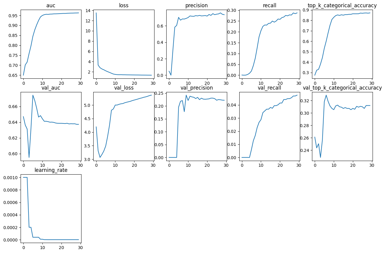
可视化训练期间的模型指标

我们使用上面定义的函数来查看训练期间的模型指标。

plot_history_metrics(conv_model_history)

png

在测试数据上评估模型

loss, accuracy, auc, precision, recall = conv_model.evaluate(test_dataset)
print(f"Loss : {loss}")
print(f"Top 3 Categorical Accuracy : {accuracy}")
print(f"Area under the Curve (ROC) : {auc}")
print(f"Precision : {precision}")
print(f"Recall : {recall}")


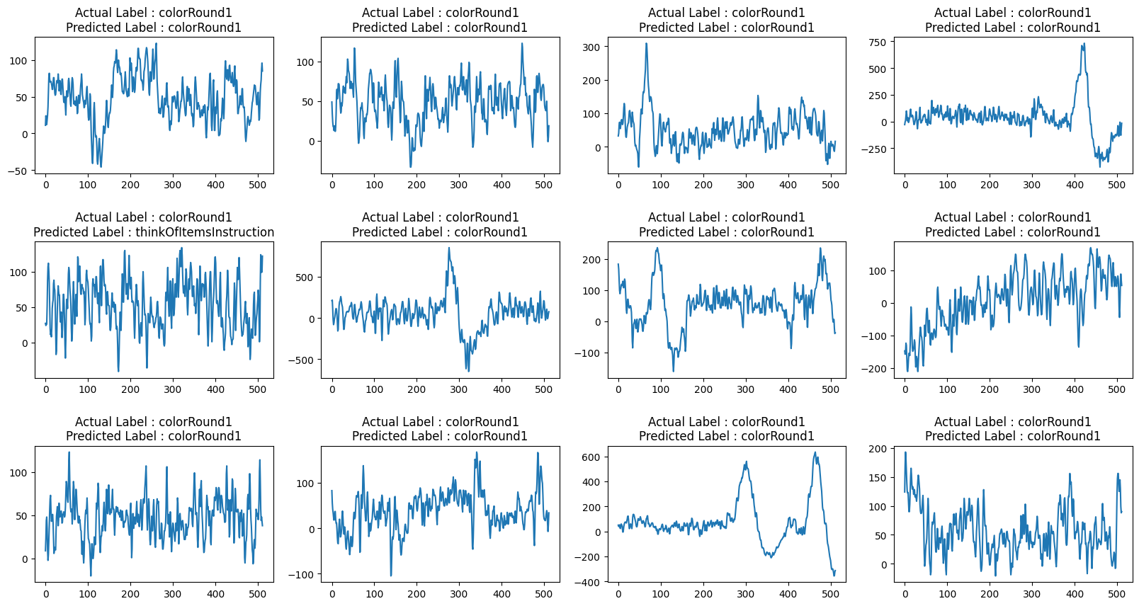
def view_evaluated_eeg_plots(model):
    start_index = random.randint(10, len(eeg))
    end_index = start_index + 11
    data = eeg.loc[start_index:end_index, "raw_values"]
    data_array = [scaler.fit_transform(np.asarray(i).reshape(-1, 1)) for i in data]
    data_array = [np.asarray(data_array).astype(np.float32).reshape(-1, 512, 1)]
    original_labels = eeg.loc[start_index:end_index, "label"]
    predicted_labels = np.argmax(model.predict(data_array, verbose=0), axis=1)
    original_labels = [
        le.inverse_transform(np.array(label).reshape(-1))[0]
        for label in original_labels
    ]
    predicted_labels = [
        le.inverse_transform(np.array(label).reshape(-1))[0]
        for label in predicted_labels
    ]
    total_plots = 12
    cols = total_plots // 3
    rows = total_plots // cols
    if total_plots % cols != 0:
        rows += 1
    pos = range(1, total_plots + 1)
    fig = plt.figure(figsize=(20, 10))
    for i, (plot_data, og_label, pred_label) in enumerate(
        zip(data, original_labels, predicted_labels)
    ):
        plt.subplot(rows, cols, pos[i])
        plt.plot(plot_data)
        plt.title(f"Actual Label : {og_label}\nPredicted Label : {pred_label}")
        fig.subplots_adjust(hspace=0.5)
    plt.show()


view_evaluated_eeg_plots(conv_model)

 24/24 ━━━━━━━━━━━━━━━━━━━━ 0s 4ms/step - auc: 0.6438 - loss: 5.3150 - precision: 0.2589 - recall: 0.0565 - top_k_categorical_accuracy: 0.3281
Loss : 5.366718769073486
Top 3 Categorical Accuracy : 0.6372398138046265
Area under the Curve (ROC) : 0.222570538520813
Precision : 0.04752342775464058
Recall : 0.311914324760437

W0000 00:00:1699421785.101645    4408 graph_launch.cc:671] Fallback to op-by-op mode because memset node breaks graph update

png