用于脑机接口的脑电图信号分类
作者: Okba Bekhelifi
创建日期 2025/01/08
最后修改日期 2025/01/08
描述: 基于 Transformer 的脑电图信号分类模型,用于脑机接口。

简介
本教程将解释如何构建一个基于 Transformer 的神经网络来分类脑机接口 (BCI) 中稳态视觉诱发电位 (SSVEPs) 实验记录的脑电图 (EEG) 数据,应用于脑控拼写器。
本教程重现了 SSVEPFormer 研究 [1] 中的一个实验(arXiv 预印本 / 同行评审论文)。该模型是第一个用于 SSVEP 数据分类的 Transformer 模型,我们将在 Nakanishi 等人 [2] 的公开数据集中对其进行测试,该数据集是论文中的数据集 1。
该过程遵循跨被试分类实验。给定数据集中有 N 个被试的数据,训练集包含 N-1 个被试的数据,而剩余的单个被试数据用于测试。训练集不包含任何来自测试被试的样本。这样我们就构建了一个真正的被试无关模型。在从预处理到训练的所有处理操作中,我们都保持与原始论文相同的参数和设置。
本教程首先对 BCI 和数据集进行简要描述,然后我们将通过以下部分深入技术细节:- 设置和导入。- 数据集下载和提取。- 数据预处理:EEG 数据滤波、分段以及原始和滤波数据的可视化,以及一个表现良好的参与者的频率响应。- 层和模型创建。- 评估:以单个被试数据分类为例,然后是全部被试数据分类。- 可视化:我们展示了在三种不同的 GPU 上,Keras 3 可用的后端(JAX、Tensorflow 和 PyTorch)之间的训练和推理时间比较结果。- 结论:最终讨论和注意事项。
数据集描述
BCI 和 SSVEP
BCI 提供仅通过大脑活动进行交流的能力,这可以通过外源性刺激来实现,外源性刺激会产生表明被试意图的特定反应。当用户专注于目标刺激时,这些反应会被引发。我们可以通过在显示器上以网格状呈现一组选项给被试来使用视觉刺激,每次选择一个命令。每个刺激都会以固定的频率和相位闪烁,在枕叶和枕顶叶皮层区域(视觉皮层)记录的 EEG 将在被试注视的刺激相关频率上显示出更高的功率。这种类型的 BCI 范式称为稳态视觉诱发电位 (SSVEPs),由于其可靠性、高分类性能和快速性(1 秒的 EEG 就足够发出一个命令),已广泛应用于多种应用。存在其他类型的脑响应,不需要外部刺激,但它们不太可靠。演示视频
本教程使用 12 命令(类别)的公开 SSVEP 数据集 [2],界面如下,模拟拨打电话号码。
该数据集记录了 10 名参与者的脑电图,每位参与者都面对上述 12 种 SSVEP 刺激(A)。刺激频率范围为 9.25Hz 至 14.75 Hz,步长为 0.5Hz,相位范围为 0 至 1.5 π,每行步长为 0.5 π(B)。EEG 信号使用 8 个电极(通道)(PO7、PO3、POz、PO4、PO8、O1、Oz、O2)采集,采样频率为 2048 Hz,然后存储的数据被降采样到 256 Hz。被试完成了 15 个记录块,每个块由 12 次随机排序的刺激(每个类别 1 次)组成,每次持续 4 秒。总共,每位被试进行了 180 次试验。
设置
选择 JAX 后端
import os

os.environ["KERAS_BACKEND"] = "jax"
安装依赖项
!pip install -q numpy
!pip install -q scipy
!pip install -q matplotlib
导入
# deep learning libraries
from keras import backend as K
from keras import layers
import keras

# visualization and signal processing imports
import matplotlib.pyplot as plt
import tensorflow as tf
import numpy as np
from scipy.signal import butter, filtfilt
from scipy.io import loadmat

# setting the backend, seed and Keras channel format
K.set_image_data_format("channels_first")
keras.utils.set_random_seed(42)
下载并解压数据集
Nakanishi 等人 2015 数据集仓库
!curl -O https://sccn.ucsd.edu/download/cca_ssvep.zip
!unzip cca_ssvep.zip
  % Total    % Received % Xferd  Average Speed   Time    Time     Time  Current
                                 Dload  Upload   Total   Spent    Left  Speed
0 0 0 0 0 0 0 0 –:–:– –:–:– –:–:– 0 0 0 0 0 0 0 0 0 –:–:– –:–:– –:–:– 0
0 145M 0 49152 0 0 40897 0 1:02:11 0:00:01 1:02:10 40891
1 145M 1 2480k 0 0 1140k 0 0:02:10 0:00:02 0:02:08 1140k
9 145M 9 13.4M 0 0 4371k 0 0:00:34 0:00:03 0:00:31 4371k
17 145M 17 25.9M 0 0 6201k 0 0:00:24 0:00:04 0:00:20 6200k
25 145M 25 37.2M 0 0 7398k 0 0:00:20 0:00:05 0:00:15 7632k
33 145M 33 48.9M 0 0 8052k 0 0:00:18 0:00:06 0:00:12 9972k
41 145M 41 60.3M 0 0 8586k 0 0:00:17 0:00:07 0:00:10 11.5M
49 145M 49 71.9M 0 0 9014k 0 0:00:16 0:00:08 0:00:08 11.6M
57 145M 57 84.2M 0 0 9423k 0 0:00:15 0:00:09 0:00:06 11.9M
66 145M 66 96.5M 0 0 9709k 0 0:00:15 0:00:10 0:00:05 11.8M
74 145M 74 108M 0 0 9938k 0 0:00:14 0:00:11 0:00:03 12.0M
82 145M 82 119M 0 0 9.8M 0 0:00:14 0:00:12 0:00:02 11.8M
90 145M 90 131M 0 0 9.9M 0 0:00:14 0:00:13 0:00:01 11.8M
98 145M 98 142M 0 0 10.0M 0 0:00:14 0:00:14 –:–:– 11.7M 100 145M 100 145M 0 0 10.1M 0 0:00:14 0:00:14 –:–:– 11.7M
Archive:  cca_ssvep.zip
   creating: cca_ssvep/
  inflating: cca_ssvep/s4.mat
  inflating: cca_ssvep/s5.mat
  inflating: cca_ssvep/s3.mat
  inflating: cca_ssvep/s7.mat
  inflating: cca_ssvep/chan_locs.pdf
  inflating: cca_ssvep/readme.txt
  inflating: cca_ssvep/s2.mat
  inflating: cca_ssvep/s8.mat
inflating: cca_ssvep/s10.mat
inflating: cca_ssvep/s9.mat
  inflating: cca_ssvep/s6.mat
  inflating: cca_ssvep/s1.mat
预处理
遵循的预处理步骤是:首先读取每个被试的 EEG 数据,然后在大多数有用信息所在的频率区间内滤波原始数据,然后我们选择从刺激开始(由于视觉系统造成的延迟,我们将在刺激开始时间上增加 135 毫秒)的固定持续时间信号。最后,将所有被试的数据连接成一个形状为 [被试数 x 样本数 x 通道数 x 试验数] 的单个张量。数据标签也按照实验中的试验顺序连接,将是一个形状为 [被试数 x 试验数] 的矩阵(此处通道数指电极,我们在整个教程中都使用此表示法)。
def raw_signal(folder, fs=256, duration=1.0, onset=0.135):
    """selecting a 1-second segment of the raw EEG signal for
    subject 1.
    """
    onset = 38 + int(onset * fs)
    end = int(duration * fs)
    data = loadmat(f"{folder}/s1.mat")
    # samples, channels, trials, targets
    eeg = data["eeg"].transpose((2, 1, 3, 0))
    # segment data
    eeg = eeg[onset : onset + end, :, :, :]
    return eeg


def segment_eeg(
    folder, elecs=None, fs=256, duration=1.0, band=[5.0, 45.0], order=4, onset=0.135
):
    """Filtering and segmenting EEG signals for all subjects."""
    n_subejects = 10
    onset = 38 + int(onset * fs)
    end = int(duration * fs)
    X, Y = [], []  # empty data and labels

    for subj in range(1, n_subejects + 1):
        data = loadmat(f"{data_folder}/s{subj}.mat")
        # samples, channels, trials, targets
        eeg = data["eeg"].transpose((2, 1, 3, 0))
        # filter data
        eeg = filter_eeg(eeg, fs=fs, band=band, order=order)
        # segment data
        eeg = eeg[onset : onset + end, :, :, :]
        # reshape labels
        samples, channels, blocks, targets = eeg.shape
        y = np.tile(np.arange(1, targets + 1), (blocks, 1))
        y = y.reshape((1, blocks * targets), order="F")

        X.append(eeg.reshape((samples, channels, blocks * targets), order="F"))
        Y.append(y)

    X = np.array(X, dtype=np.float32, order="F")
    Y = np.array(Y, dtype=np.float32).squeeze()

    return X, Y


def filter_eeg(data, fs=256, band=[5.0, 45.0], order=4):
    """Filter EEG signal using a zero-phase IIR filter"""
    B, A = butter(order, np.array(band) / (fs / 2), btype="bandpass")
    return filtfilt(B, A, data, axis=0)
将数据分段到时期
data_folder = os.path.abspath("./cca_ssvep")
band = [8, 64]  # low-frequency / high-frequency cutoffS
order = 4  # filter order
fs = 256  # sampling frequency
duration = 1.0  # 1 second

# raw signal
X_raw = raw_signal(data_folder, fs=fs, duration=duration)
print(
    f"A single subject raw EEG (X_raw) shape: {X_raw.shape} [Samples x Channels x Blocks x Targets]"
)

# segmented signal
X, Y = segment_eeg(data_folder, band=band, order=order, fs=fs, duration=duration)
print(
    f"Full training data (X) shape: {X.shape} [Subject x Samples x Channels x Trials]"
)
print(f"data labels (Y) shape:        {Y.shape} [Subject x Trials]")

samples = X.shape[1]
time = np.linspace(0.0, samples / fs, samples) * 1000
A single subject raw EEG (X_raw) shape: (256, 8, 15, 12) [Samples x Channels x Blocks x Targets]

Full training data (X) shape: (10, 256, 8, 180) [Subject x Samples x Channels x Trials]
data labels (Y) shape:        (10, 180) [Subject x Trials]
可视化 EEG 信号
EEG 时域信号
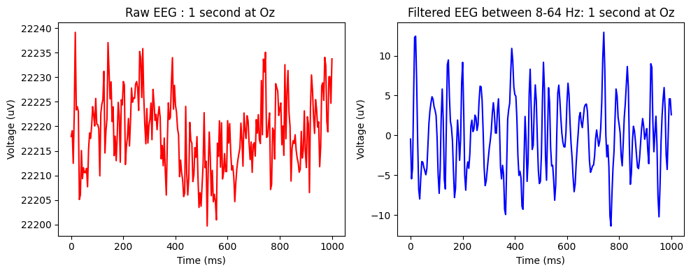
原始 EEG 与滤波 EEG。图示了参与者 s1 在 Oz(视觉皮层中心电极,头后部)的同一 1 秒录制。左侧是记录的原始 EEG,右侧是在 [8, 64] Hz 频率带内滤波后的 EEG。我们看到噪声减少,幅度值标准化到自然 EEG 范围。
elec = 6  # Oz channel

x_label = "Time (ms)"
y_label = "Voltage (uV)"
# Create subplots
fig, (ax1, ax2) = plt.subplots(1, 2, figsize=(10, 4))

# Plot data on the first subplot
ax1.plot(time, X_raw[:, elec, 0, 0], "r-")
ax1.set_xlabel(x_label)
ax1.set_ylabel(y_label)
ax1.set_title("Raw EEG : 1 second at Oz ")

# Plot data on the second subplot
ax2.plot(time, X[0, :, elec, 0], "b-")
ax2.set_xlabel(x_label)
ax2.set_ylabel(y_label)
ax2.set_title("Filtered EEG between 8-64 Hz: 1 second at Oz")

# Adjust spacing between subplots
plt.tight_layout()

# Show the plot
plt.show()
EEG 频率表示
使用 Welch 方法,我们可视化一个表现良好的参与者在 Oz 电极上进行 4 秒 EEG 录制的频率功率,针对每个刺激。红色的峰值表示刺激的基频和二次谐波(基频的两倍)。我们看到清晰的峰值,表明该参与者反应良好,这意味着该参与者是 SSVEP BCI 控制的良好候选者。在许多情况下,峰值很弱或不存在,这意味着参与者没有正确完成任务。

创建层和模型
以跨框架自定义组件的方式创建层。在 SSVEPFormer 中,数据首先通过快速傅里叶变换 (FFT) 转换到频域,以构建一个复数频谱表示,由固定频带内的频率和相位信息的拼接组成。为了保持模型的端到端格式,我们将复数频谱变换实现为非可训练层。
 与 Transformer 架构不同,SSVEPFormer 不包含位置编码/嵌入层,取而代之的是一个通道组合块,其中包含一个核大小为 1 的 Conv1D 层,具有双倍输入通道(电极数量加倍)的滤波器数量,以及 LayerNorm、Gelu 激活和 dropout。与 Transformer 的另一个不同之处在于缺少具有注意力机制的多头注意力层。模型编码器包含两个相同且连续的块。每个块有两个子块:CNN 模块和 MLP 模块。CNN 模块由 LayerNorm、Conv1D(具有与通道组合相同的滤波器数量)、LayerNorm、Gelu、Dropout 和残差连接组成。MLP 模块由 LayerNorm、Dense 层、Gelu、Dropout 和残差连接组成。Dense 层分别应用于每个通道。模型的最后一个块是 MLP 头,包含 Flatten 层、Dropout、Dense、LayerNorm、Gelu、Dropout 和带有 softmax 激活的 Dense 层。根据原始论文的说法,所有可训练权重都初始化为均值为 0、标准差为 0.01 的正态分布。
class ComplexSpectrum(keras.layers.Layer):
    def __init__(self, nfft=512, fft_start=8, fft_end=64):
        super().__init__()
        self.nfft = nfft
        self.fft_start = fft_start
        self.fft_end = fft_end

    def call(self, x):
        samples = x.shape[-1]
        x = keras.ops.rfft(x, fft_length=self.nfft)
        real = x[0] / samples
        imag = x[1] / samples
        real = real[:, :, self.fft_start : self.fft_end]
        imag = imag[:, :, self.fft_start : self.fft_end]
        x = keras.ops.concatenate((real, imag), axis=-1)
        return x


class ChannelComb(keras.layers.Layer):
    def __init__(self, n_channels, drop_rate=0.5):
        super().__init__()
        self.conv = layers.Conv1D(
            2 * n_channels,
            1,
            padding="same",
            kernel_initializer=keras.initializers.RandomNormal(
                mean=0.0, stddev=0.01, seed=None
            ),
        )
        self.normalization = layers.LayerNormalization()
        self.activation = layers.Activation(activation="gelu")
        self.drop = layers.Dropout(drop_rate)

    def call(self, x):
        x = self.conv(x)
        x = self.normalization(x)
        x = self.activation(x)
        x = self.drop(x)
        return x


class ConvAttention(keras.layers.Layer):
    def __init__(self, n_channels, drop_rate=0.5):
        super().__init__()
        self.norm = layers.LayerNormalization()
        self.conv = layers.Conv1D(
            2 * n_channels,
            31,
            padding="same",
            kernel_initializer=keras.initializers.RandomNormal(
                mean=0.0, stddev=0.01, seed=None
            ),
        )
        self.activation = layers.Activation(activation="gelu")
        self.drop = layers.Dropout(drop_rate)

    def call(self, x):
        input = x
        x = self.norm(x)
        x = self.conv(x)
        x = self.activation(x)
        x = self.drop(x)
        x = x + input
        return x


class ChannelMLP(keras.layers.Layer):
    def __init__(self, n_features, drop_rate=0.5):
        super().__init__()
        self.norm = layers.LayerNormalization()
        self.mlp = layers.Dense(
            2 * n_features,
            kernel_initializer=keras.initializers.RandomNormal(
                mean=0.0, stddev=0.01, seed=None
            ),
        )
        self.activation = layers.Activation(activation="gelu")
        self.drop = layers.Dropout(drop_rate)
        self.cat = layers.Concatenate(axis=1)

    def call(self, x):
        input = x
        channels = x.shape[1]  # x shape : NCF
        x = self.norm(x)
        output_channels = []
        for i in range(channels):
            c = self.mlp(x[:, :, i])
            c = layers.Reshape([1, -1])(c)
            output_channels.append(c)
        x = self.cat(output_channels)
        x = self.activation(x)
        x = self.drop(x)
        x = x + input
        return x


class Encoder(keras.layers.Layer):
    def __init__(self, n_channels, n_features, drop_rate=0.5):
        super().__init__()
        self.attention1 = ConvAttention(n_channels, drop_rate=drop_rate)
        self.mlp1 = ChannelMLP(n_features, drop_rate=drop_rate)
        self.attention2 = ConvAttention(n_channels, drop_rate=drop_rate)
        self.mlp2 = ChannelMLP(n_features, drop_rate=drop_rate)

    def call(self, x):
        x = self.attention1(x)
        x = self.mlp1(x)
        x = self.attention2(x)
        x = self.mlp2(x)
        return x


class MlpHead(keras.layers.Layer):
    def __init__(self, n_classes, drop_rate=0.5):
        super().__init__()
        self.flatten = layers.Flatten()
        self.drop = layers.Dropout(drop_rate)
        self.linear1 = layers.Dense(
            6 * n_classes,
            kernel_initializer=keras.initializers.RandomNormal(
                mean=0.0, stddev=0.01, seed=None
            ),
        )
        self.norm = layers.LayerNormalization()
        self.activation = layers.Activation(activation="gelu")
        self.drop2 = layers.Dropout(drop_rate)
        self.linear2 = layers.Dense(
            n_classes,
            kernel_initializer=keras.initializers.RandomNormal(
                mean=0.0, stddev=0.01, seed=None
            ),
        )

    def call(self, x):
        x = self.flatten(x)
        x = self.drop(x)
        x = self.linear1(x)
        x = self.norm(x)
        x = self.activation(x)
        x = self.drop2(x)
        x = self.linear2(x)
        return x
使用上述层创建顺序模型
def create_ssvepformer(
    input_shape, fs, resolution, fq_band, n_channels, n_classes, drop_rate
):
    nfft = round(fs / resolution)
    fft_start = int(fq_band[0] / resolution)
    fft_end = int(fq_band[1] / resolution) + 1
    n_features = fft_end - fft_start

    model = keras.Sequential(
        [
            keras.Input(shape=input_shape),
            ComplexSpectrum(nfft, fft_start, fft_end),
            ChannelComb(n_channels=n_channels, drop_rate=drop_rate),
            Encoder(n_channels=n_channels, n_features=n_features, drop_rate=drop_rate),
            Encoder(n_channels=n_channels, n_features=n_features, drop_rate=drop_rate),
            MlpHead(n_classes=n_classes, drop_rate=drop_rate),
            layers.Activation(activation="softmax"),
        ]
    )

    return model
评估
# Training settings same as the original paper
BATCH_SIZE = 128
EPOCHS = 100
LR = 0.001  # learning rate
WD = 0.001  # weight decay
MOMENTUM = 0.9
DROP_RATE = 0.5

resolution = 0.25
从整个数据集中,我们为每个被试的评估选择折叠。构建一个用于训练和测试数据的 tf dataset 对象,创建模型并使用 SGD 优化器启动训练。
def concatenate_subjects(x, y, fold):
    X = np.concatenate([x[idx] for idx in fold], axis=-1)
    Y = np.concatenate([y[idx] for idx in fold], axis=-1)
    X = X.transpose((2, 1, 0))  # trials x channels x samples
    return X, Y - 1  # transform labels to values from 0...11


def evaluate_subject(
    x_train,
    y_train,
    x_val,
    y_val,
    input_shape,
    fs=256,
    resolution=0.25,
    band=[8, 64],
    channels=8,
    n_classes=12,
    drop_rate=DROP_RATE,
):

    train_dataset = (
        tf.data.Dataset.from_tensor_slices((x_train, y_train))
        .batch(BATCH_SIZE)
        .prefetch(tf.data.AUTOTUNE)
    )

    test_dataset = (
        tf.data.Dataset.from_tensor_slices((x_val, y_val))
        .batch(BATCH_SIZE)
        .prefetch(tf.data.AUTOTUNE)
    )

    model = create_ssvepformer(
        input_shape, fs, resolution, band, channels, n_classes, drop_rate
    )
    sgd = keras.optimizers.SGD(learning_rate=LR, momentum=MOMENTUM, weight_decay=WD)

    model.compile(
        loss="sparse_categorical_crossentropy",
        optimizer=sgd,
        metrics=["accuracy"],
        jit_compile=True,
    )

    history = model.fit(
        train_dataset,
        batch_size=BATCH_SIZE,
        epochs=EPOCHS,
        validation_data=test_dataset,
        verbose=0,
    )
    loss, acc = model.evaluate(test_dataset)
    return acc * 100
运行评估
channels = X.shape[2]
samples = X.shape[1]
input_shape = (channels, samples)
n_classes = 12

model = create_ssvepformer(
    input_shape, fs, resolution, band, channels, n_classes, DROP_RATE
)
model.summary()
Model: "sequential"
┏━━━━━━━━━━━━━━━━━━━━━━━━━━━━━━━━━━━━━━┳━━━━━━━━━━━━━━━━━━━━━━━━━━━━━┳━━━━━━━━━━━━━━━━━┓
┃ Layer (type)                         ┃ Output Shape                ┃         Param # ┃
┡━━━━━━━━━━━━━━━━━━━━━━━━━━━━━━━━━━━━━━╇━━━━━━━━━━━━━━━━━━━━━━━━━━━━━╇━━━━━━━━━━━━━━━━━┩
│ complex_spectrum (ComplexSpectrum)   │ (None, 8, 450)              │               0 │
├──────────────────────────────────────┼─────────────────────────────┼─────────────────┤
│ channel_comb (ChannelComb)           │ (None, 16, 450)             │           1,044 │
├──────────────────────────────────────┼─────────────────────────────┼─────────────────┤
│ encoder (Encoder)                    │ (None, 16, 450)             │          34,804 │
├──────────────────────────────────────┼─────────────────────────────┼─────────────────┤
│ encoder_1 (Encoder)                  │ (None, 16, 450)             │          34,804 │
├──────────────────────────────────────┼─────────────────────────────┼─────────────────┤
│ mlp_head (MlpHead)                   │ (None, 12)                  │         519,492 │
├──────────────────────────────────────┼─────────────────────────────┼─────────────────┤
│ activation_10 (Activation)           │ (None, 12)                  │               0 │
└──────────────────────────────────────┴─────────────────────────────┴─────────────────┘
Total params: 590,144 (2.25 MB)
Trainable params: 590,144 (2.25 MB)
Non-trainable params: 0 (0.00 B)
基于留一被试交叉验证的数据划分方案对所有被试进行评估
accs = np.zeros(10)

for subject in range(10):
    print(f"Testing subject: {subject+ 1}")

    # create train / test folds
    folds = np.delete(np.arange(10), subject)
    train_index = folds
    test_index = [subject]

    # create data split for each subject
    x_train, y_train = concatenate_subjects(X, Y, train_index)
    x_val, y_val = concatenate_subjects(X, Y, test_index)

    # train and evaluate a fold and compute the time it takes
    acc = evaluate_subject(x_train, y_train, x_val, y_val, input_shape)

    accs[subject] = acc

print(f"\nAccuracy Across Subjects: {accs.mean()} % std: {np.std(accs)}")
Testing subject: 1

WARNING: All log messages before absl::InitializeLog() is called are written to STDERR
I0000 00:00:1737801392.665434    1425 cuda_executor.cc:1015] successful NUMA node read from SysFS had negative value (-1), but there must be at least one NUMA node, so returning NUMA node zero. See more at https://github.com/torvalds/linux/blob/v6.0/Documentation/ABI/testing/sysfs-bus-pci#L344-L355
I0000 00:00:1737801393.156241    1425 cuda_executor.cc:1015] successful NUMA node read from SysFS had negative value (-1), but there must be at least one NUMA node, so returning NUMA node zero. See more at https://github.com/torvalds/linux/blob/v6.0/Documentation/ABI/testing/sysfs-bus-pci#L344-L355
I0000 00:00:1737801393.156492    1425 cuda_executor.cc:1015] successful NUMA node read from SysFS had negative value (-1), but there must be at least one NUMA node, so returning NUMA node zero. See more at https://github.com/torvalds/linux/blob/v6.0/Documentation/ABI/testing/sysfs-bus-pci#L344-L355
I0000 00:00:1737801393.160002    1425 cuda_executor.cc:1015] successful NUMA node read from SysFS had negative value (-1), but there must be at least one NUMA node, so returning NUMA node zero. See more at https://github.com/torvalds/linux/blob/v6.0/Documentation/ABI/testing/sysfs-bus-pci#L344-L355
I0000 00:00:1737801393.160279    1425 cuda_executor.cc:1015] successful NUMA node read from SysFS had negative value (-1), but there must be at least one NUMA node, so returning NUMA node zero. See more at https://github.com/torvalds/linux/blob/v6.0/Documentation/ABI/testing/sysfs-bus-pci#L344-L355
I0000 00:00:1737801393.160421    1425 cuda_executor.cc:1015] successful NUMA node read from SysFS had negative value (-1), but there must be at least one NUMA node, so returning NUMA node zero. See more at https://github.com/torvalds/linux/blob/v6.0/Documentation/ABI/testing/sysfs-bus-pci#L344-L355
I0000 00:00:1737801393.168480    1425 cuda_executor.cc:1015] successful NUMA node read from SysFS had negative value (-1), but there must be at least one NUMA node, so returning NUMA node zero. See more at https://github.com/torvalds/linux/blob/v6.0/Documentation/ABI/testing/sysfs-bus-pci#L344-L355
I0000 00:00:1737801393.168667    1425 cuda_executor.cc:1015] successful NUMA node read from SysFS had negative value (-1), but there must be at least one NUMA node, so returning NUMA node zero. See more at https://github.com/torvalds/linux/blob/v6.0/Documentation/ABI/testing/sysfs-bus-pci#L344-L355
I0000 00:00:1737801393.168908    1425 cuda_executor.cc:1015] successful NUMA node read from SysFS had negative value (-1), but there must be at least one NUMA node, so returning NUMA node zero. See more at https://github.com/torvalds/linux/blob/v6.0/Documentation/ABI/testing/sysfs-bus-pci#L344-L355
1/2 ━━━━━━━━━━ [37m━━━━━━━━━━ 0s 7ms/step - accuracy: 0.5938 - loss: 1.2483
2/2 ━━━━━━━━━━━━━━━━━━━━ 0s 39ms/step - accuracy: 0.5868 - loss: 1.3010
Testing subject: 2
1/2 ━━━━━━━━━━[37m━━━━━━━━━━ 0s 7ms/step - accuracy: 0.5469 - loss: 1.5270
2/2 ━━━━━━━━━━━━━━━━━━━━ 0s 7ms/step - accuracy: 0.5119 - loss: 1.5974
Testing subject: 3
1/2 ━━━━━━━━━━[37m━━━━━━━━━━ 0s 7ms/step - accuracy: 0.7266 - loss: 0.8867
2/2 ━━━━━━━━━━━━━━━━━━━━ 0s 7ms/step - accuracy: 0.6903 - loss: 1.0117
Testing subject: 4
1/2 ━━━━━━━━━━[37m━━━━━━━━━━ 0s 7ms/step - accuracy: 0.9688 - loss: 0.1574
2/2 ━━━━━━━━━━━━━━━━━━━━ 0s 8ms/step - accuracy: 0.9637 - loss: 0.1487
Testing subject: 5
1/2 ━━━━━━━━━━[37m━━━━━━━━━━ 0s 7ms/step - accuracy: 0.9375 - loss: 0.2184
2/2 ━━━━━━━━━━━━━━━━━━━━ 0s 7ms/step - accuracy: 0.9458 - loss: 0.1887
Testing subject: 6
1/2 ━━━━━━━━━━[37m━━━━━━━━━━ 0s 12ms/step - accuracy: 0.9688 - loss: 0.1117
2/2 ━━━━━━━━━━━━━━━━━━━━ 0s 10ms/step - accuracy: 0.9674 - loss: 0.1018
Testing subject: 7
1/2 ━━━━━━━━━━[37m━━━━━━━━━━ 0s 7ms/step - accuracy: 0.9141 - loss: 0.2639
2/2 ━━━━━━━━━━━━━━━━━━━━ 0s 7ms/step - accuracy: 0.9158 - loss: 0.2592
Testing subject: 8
1/2 ━━━━━━━━━━[37m━━━━━━━━━━ 0s 9ms/step - accuracy: 0.9922 - loss: 0.0562
2/2 ━━━━━━━━━━━━━━━━━━━━ 0s 20ms/step - accuracy: 0.9937 - loss: 0.0518
Testing subject: 9
1/2 ━━━━━━━━━━[37m━━━━━━━━━━ 0s 7ms/step - accuracy: 0.9844 - loss: 0.0669
2/2 ━━━━━━━━━━━━━━━━━━━━ 0s 8ms/step - accuracy: 0.9837 - loss: 0.0701
Testing subject: 10
1/2 ━━━━━━━━━━[37m━━━━━━━━━━ 0s 10ms/step - accuracy: 0.9219 - loss: 0.3438
2/2 ━━━━━━━━━━━━━━━━━━━━ 0s 18ms/step - accuracy: 0.8999 - loss: 0.4543
Accuracy Across Subjects: 84.11111384630203 % std: 17.575586372993953
就这样!我们看到一些在训练集中没有数据的被试仍然可以达到近乎 100% 的正确命令,而另一些则表现不佳,准确率在 50% 左右。在原始论文中使用 PyTorch 时,平均准确率为 84.04%,标准差为 17.37。考虑到深度学习的随机性,我们达到了相同的值。
可视化
在 Colab 免费/Pro/Pro+ 可用的三个 GPU(T4、L4、A100)上,比较 Jax、Tensorflow 和 PyTorch 这几种后端之间的训练和推理时间。
训练时间

推理时间

Jax 后端在所有 GPU 上的训练和推理方面表现最佳,PyTorch 由于禁用了 jit 编译选项而非常缓慢,因为 FFT 计算的复杂数据类型不支持 PyTorch jit 编译器。
致谢
我感谢 Chris Perry X @GoogleColab 为这项工作提供 GPU 计算支持。
参考文献
[1] Chen, J. et al. (2023) ‘A transformer-based deep neural network model for SSVEP classification’, Neural Networks, 164, pp. 521–534. 可用地址:https://doi.org/10.1016/j.neunet.2023.04.045。
[2] Nakanishi, M. et al. (2015) ‘A Comparison Study of Canonical Correlation Analysis Based Methods for Detecting Steady-State Visual Evoked Potentials’, Plos One, 10(10), p. e0140703. 可用地址:https://doi.org/10.1371/journal.pone.0140703