使用图神经网络和 LSTM 进行交通流量预测
作者: Arash Khodadadi
创建日期 2021/12/28
最后修改日期 2023/11/22
描述: 这个例子演示了如何在图上进行时间序列预测。

简介
本示例展示了如何使用图神经网络和 LSTM 来预测交通状况。具体来说,我们有兴趣在给定一段道路路段的交通速度历史记录的情况下,预测这些路段交通速度的未来值。
解决此问题的一种流行方法是将每个道路路段的交通速度视为单独的时间序列,并使用同一时间序列的过去值来预测每个时间序列的未来值。
然而,这种方法忽略了一个道路路段的交通速度对其邻近路段的依赖性。为了能够考虑一系列相邻道路上交通速度之间的复杂交互,我们可以将交通网络定义为图,并将交通速度视为该图上的信号。在本示例中,我们将实现一个能够处理图上的时间序列数据的神经网络架构。首先,我们将展示如何处理数据并创建用于图上预测的 tf.data.Dataset。然后,我们将实现一个使用图卷积和 LSTM 层在图上执行预测的模型。
数据处理和网络架构受到以下论文的启发
Yu, Bing, Haoteng Yin, and Zhanxing Zhu. "Spatio-temporal graph convolutional networks: a deep learning framework for traffic forecasting." Proceedings of the 27th International Joint Conference on Artificial Intelligence, 2018. (github)
设置
import os

os.environ["KERAS_BACKEND"] = "tensorflow"

import pandas as pd
import numpy as np
import typing
import matplotlib.pyplot as plt

import tensorflow as tf
import keras
from keras import layers
from keras import ops
数据准备
数据描述
我们使用一个名为 PeMSD7 的真实世界交通速度数据集。我们使用 Yu 等人(2018 年)收集和准备的版本,该版本可在此 处找到。
数据包含两个文件
PeMSD7_W_228.csv包含加利福尼亚州第 7 区 228 个站点之间的距离。PeMSD7_V_228.csv包含 2012 年 5 月和 6 月工作日收集的这些站点的交通速度。
数据集的完整描述可以在 Yu 等人(2018 年)中找到。
加载数据
url = "https://github.com/VeritasYin/STGCN_IJCAI-18/raw/master/dataset/PeMSD7_Full.zip"
data_dir = keras.utils.get_file(origin=url, extract=True, archive_format="zip")
data_dir = data_dir.rstrip("PeMSD7_Full.zip")

route_distances = pd.read_csv(
    os.path.join(data_dir, "PeMSD7_W_228.csv"), header=None
).to_numpy()
speeds_array = pd.read_csv(
    os.path.join(data_dir, "PeMSD7_V_228.csv"), header=None
).to_numpy()

print(f"route_distances shape={route_distances.shape}")
print(f"speeds_array shape={speeds_array.shape}")
route_distances shape=(228, 228)
speeds_array shape=(12672, 228)
对道路进行子采样
为了减小问题规模并加快训练速度,我们将仅使用数据集中 228 条道路中的 26 条进行采样。我们选择道路的方式是从道路 0 开始,选择离它最近的 5 条道路,然后继续此过程,直到获得 25 条道路。您可以选择任何其他道路子集。我们之所以这样选择道路,是为了增加具有相关速度时间序列的道路的可能性。sample_routes 包含所选道路的 ID。
sample_routes = [
    0,
    1,
    4,
    7,
    8,
    11,
    15,
    108,
    109,
    114,
    115,
    118,
    120,
    123,
    124,
    126,
    127,
    129,
    130,
    132,
    133,
    136,
    139,
    144,
    147,
    216,
]
route_distances = route_distances[np.ix_(sample_routes, sample_routes)]
speeds_array = speeds_array[:, sample_routes]

print(f"route_distances shape={route_distances.shape}")
print(f"speeds_array shape={speeds_array.shape}")
route_distances shape=(26, 26)
speeds_array shape=(12672, 26)
数据可视化
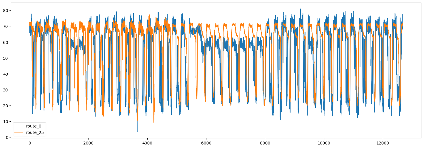
以下是两条道路的交通速度时间序列
plt.figure(figsize=(18, 6))
plt.plot(speeds_array[:, [0, -1]])
plt.legend(["route_0", "route_25"])
<matplotlib.legend.Legend at 0x7f5a870b2050>
我们还可以可视化不同道路时间序列之间的相关性。
plt.figure(figsize=(8, 8))
plt.matshow(np.corrcoef(speeds_array.T), 0)
plt.xlabel("road number")
plt.ylabel("road number")
Text(0, 0.5, 'road number')
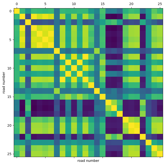
通过这个相关性热图,我们可以看到,例如,道路 4、5、6 的速度高度相关。
分割和标准化数据
接下来,我们将速度值数组分割为训练/验证/测试集,并对生成的数组进行标准化。
train_size, val_size = 0.5, 0.2


def preprocess(data_array: np.ndarray, train_size: float, val_size: float):
    """Splits data into train/val/test sets and normalizes the data.

    Args:
        data_array: ndarray of shape `(num_time_steps, num_routes)`
        train_size: A float value between 0.0 and 1.0 that represent the proportion of the dataset
            to include in the train split.
        val_size: A float value between 0.0 and 1.0 that represent the proportion of the dataset
            to include in the validation split.

    Returns:
        `train_array`, `val_array`, `test_array`
    """

    num_time_steps = data_array.shape[0]
    num_train, num_val = (
        int(num_time_steps * train_size),
        int(num_time_steps * val_size),
    )
    train_array = data_array[:num_train]
    mean, std = train_array.mean(axis=0), train_array.std(axis=0)

    train_array = (train_array - mean) / std
    val_array = (data_array[num_train : (num_train + num_val)] - mean) / std
    test_array = (data_array[(num_train + num_val) :] - mean) / std

    return train_array, val_array, test_array


train_array, val_array, test_array = preprocess(speeds_array, train_size, val_size)

print(f"train set size: {train_array.shape}")
print(f"validation set size: {val_array.shape}")
print(f"test set size: {test_array.shape}")
train set size: (6336, 26)
validation set size: (2534, 26)
test set size: (3802, 26)
创建 TensorFlow 数据集
接下来,我们将为预测问题创建数据集。预测问题可以表述如下:给定时间 t+1, t+2, ..., t+T 的道路速度值序列,我们想要预测道路速度在时间 t+T+1, ..., t+T+h 的未来值。因此,对于每个时间 t,我们模型的输入是 T 个大小为 N 的向量,目标是 h 个大小为 N 的向量,其中 N 是道路数量。
我们使用 Keras 内置函数 keras.utils.timeseries_dataset_from_array。函数 create_tf_dataset() 接收一个 numpy.ndarray 作为输入,并返回一个 tf.data.Dataset。在此函数中,input_sequence_length=T 和 forecast_horizon=h。
参数 multi_horizon 需要进一步解释。假设 forecast_horizon=3。如果 multi_horizon=True,则模型将对时间步 t+T+1, t+T+2, t+T+3 进行预测。因此,目标将具有形状 (T,3)。但如果 multi_horizon=False,模型将仅对时间步 t+T+3 进行预测,因此目标将具有形状 (T, 1)。
您可能会注意到,每个批次中的输入张量的形状为 (batch_size, input_sequence_length, num_routes, 1)。添加最后一个维度是为了使模型更加通用:在每个时间步,每条道路的输入特征可能包含多个时间序列。例如,除了历史速度值之外,还可能希望使用温度时间序列作为输入特征。然而,在本示例中,输入的最后一个维度始终为 1。
我们使用每条道路的最后 12 个速度值来预测未来 3 个时间步的速度。
batch_size = 64
input_sequence_length = 12
forecast_horizon = 3
multi_horizon = False


def create_tf_dataset(
    data_array: np.ndarray,
    input_sequence_length: int,
    forecast_horizon: int,
    batch_size: int = 128,
    shuffle=True,
    multi_horizon=True,
):
    """Creates tensorflow dataset from numpy array.

    This function creates a dataset where each element is a tuple `(inputs, targets)`.
    `inputs` is a Tensor
    of shape `(batch_size, input_sequence_length, num_routes, 1)` containing
    the `input_sequence_length` past values of the timeseries for each node.
    `targets` is a Tensor of shape `(batch_size, forecast_horizon, num_routes)`
    containing the `forecast_horizon`
    future values of the timeseries for each node.

    Args:
        data_array: np.ndarray with shape `(num_time_steps, num_routes)`
        input_sequence_length: Length of the input sequence (in number of timesteps).
        forecast_horizon: If `multi_horizon=True`, the target will be the values of the timeseries for 1 to
            `forecast_horizon` timesteps ahead. If `multi_horizon=False`, the target will be the value of the
            timeseries `forecast_horizon` steps ahead (only one value).
        batch_size: Number of timeseries samples in each batch.
        shuffle: Whether to shuffle output samples, or instead draw them in chronological order.
        multi_horizon: See `forecast_horizon`.

    Returns:
        A tf.data.Dataset instance.
    """

    inputs = keras.utils.timeseries_dataset_from_array(
        np.expand_dims(data_array[:-forecast_horizon], axis=-1),
        None,
        sequence_length=input_sequence_length,
        shuffle=False,
        batch_size=batch_size,
    )

    target_offset = (
        input_sequence_length
        if multi_horizon
        else input_sequence_length + forecast_horizon - 1
    )
    target_seq_length = forecast_horizon if multi_horizon else 1
    targets = keras.utils.timeseries_dataset_from_array(
        data_array[target_offset:],
        None,
        sequence_length=target_seq_length,
        shuffle=False,
        batch_size=batch_size,
    )

    dataset = tf.data.Dataset.zip((inputs, targets))
    if shuffle:
        dataset = dataset.shuffle(100)

    return dataset.prefetch(16).cache()


train_dataset, val_dataset = (
    create_tf_dataset(data_array, input_sequence_length, forecast_horizon, batch_size)
    for data_array in [train_array, val_array]
)

test_dataset = create_tf_dataset(
    test_array,
    input_sequence_length,
    forecast_horizon,
    batch_size=test_array.shape[0],
    shuffle=False,
    multi_horizon=multi_horizon,
)
道路图
如前所述,我们假设道路段构成一个图。PeMSD7 数据集包含道路段的距离。下一步是从这些距离创建图的邻接矩阵。遵循 Yu 等人(2018 年)(方程 10),我们假设如果两个节点之间的距离小于某个阈值,则它们之间存在一条边。
def compute_adjacency_matrix(
    route_distances: np.ndarray, sigma2: float, epsilon: float
):
    """Computes the adjacency matrix from distances matrix.

    It uses the formula in https://github.com/VeritasYin/STGCN_IJCAI-18#data-preprocessing to
    compute an adjacency matrix from the distance matrix.
    The implementation follows that paper.

    Args:
        route_distances: np.ndarray of shape `(num_routes, num_routes)`. Entry `i,j` of this array is the
            distance between roads `i,j`.
        sigma2: Determines the width of the Gaussian kernel applied to the square distances matrix.
        epsilon: A threshold specifying if there is an edge between two nodes. Specifically, `A[i,j]=1`
            if `np.exp(-w2[i,j] / sigma2) >= epsilon` and `A[i,j]=0` otherwise, where `A` is the adjacency
            matrix and `w2=route_distances * route_distances`

    Returns:
        A boolean graph adjacency matrix.
    """
    num_routes = route_distances.shape[0]
    route_distances = route_distances / 10000.0
    w2, w_mask = (
        route_distances * route_distances,
        np.ones([num_routes, num_routes]) - np.identity(num_routes),
    )
    return (np.exp(-w2 / sigma2) >= epsilon) * w_mask
函数 compute_adjacency_matrix() 返回一个布尔邻接矩阵,其中 1 表示两个节点之间存在一条边。我们使用以下类来存储图的信息。
class GraphInfo:
    def __init__(self, edges: typing.Tuple[list, list], num_nodes: int):
        self.edges = edges
        self.num_nodes = num_nodes


sigma2 = 0.1
epsilon = 0.5
adjacency_matrix = compute_adjacency_matrix(route_distances, sigma2, epsilon)
node_indices, neighbor_indices = np.where(adjacency_matrix == 1)
graph = GraphInfo(
    edges=(node_indices.tolist(), neighbor_indices.tolist()),
    num_nodes=adjacency_matrix.shape[0],
)
print(f"number of nodes: {graph.num_nodes}, number of edges: {len(graph.edges[0])}")
number of nodes: 26, number of edges: 150
网络架构
我们的图预测模型由一个图卷积层和一个 LSTM 层组成。
图卷积层
我们对图卷积层的实现类似于 此 Keras 示例中的实现。请注意,在该示例中,层的输入是一个形状为 (num_nodes,in_feat) 的 2D 张量,但在我们的示例中,层的输入是一个形状为 (num_nodes, batch_size, input_seq_length, in_feat) 的 4D 张量。图卷积层执行以下步骤
- 节点的表示在
self.compute_nodes_representation()中计算,通过将输入特征乘以self.weight。 - 邻居消息的聚合在
self.compute_aggregated_messages()中计算,首先聚合邻居的表示,然后将结果乘以self.weight。 - 该层的最终输出在
self.update()中计算,通过结合节点表示和邻居的聚合消息。
class GraphConv(layers.Layer):
    def __init__(
        self,
        in_feat,
        out_feat,
        graph_info: GraphInfo,
        aggregation_type="mean",
        combination_type="concat",
        activation: typing.Optional[str] = None,
        **kwargs,
    ):
        super().__init__(**kwargs)
        self.in_feat = in_feat
        self.out_feat = out_feat
        self.graph_info = graph_info
        self.aggregation_type = aggregation_type
        self.combination_type = combination_type
        self.weight = self.add_weight(
            initializer=keras.initializers.GlorotUniform(),
            shape=(in_feat, out_feat),
            dtype="float32",
            trainable=True,
        )
        self.activation = layers.Activation(activation)

    def aggregate(self, neighbour_representations):
        aggregation_func = {
            "sum": tf.math.unsorted_segment_sum,
            "mean": tf.math.unsorted_segment_mean,
            "max": tf.math.unsorted_segment_max,
        }.get(self.aggregation_type)

        if aggregation_func:
            return aggregation_func(
                neighbour_representations,
                self.graph_info.edges[0],
                num_segments=self.graph_info.num_nodes,
            )

        raise ValueError(f"Invalid aggregation type: {self.aggregation_type}")

    def compute_nodes_representation(self, features):
        """Computes each node's representation.

        The nodes' representations are obtained by multiplying the features tensor with
        `self.weight`. Note that
        `self.weight` has shape `(in_feat, out_feat)`.

        Args:
            features: Tensor of shape `(num_nodes, batch_size, input_seq_len, in_feat)`

        Returns:
            A tensor of shape `(num_nodes, batch_size, input_seq_len, out_feat)`
        """
        return ops.matmul(features, self.weight)

    def compute_aggregated_messages(self, features):
        neighbour_representations = tf.gather(features, self.graph_info.edges[1])
        aggregated_messages = self.aggregate(neighbour_representations)
        return ops.matmul(aggregated_messages, self.weight)

    def update(self, nodes_representation, aggregated_messages):
        if self.combination_type == "concat":
            h = ops.concatenate([nodes_representation, aggregated_messages], axis=-1)
        elif self.combination_type == "add":
            h = nodes_representation + aggregated_messages
        else:
            raise ValueError(f"Invalid combination type: {self.combination_type}.")
        return self.activation(h)

    def call(self, features):
        """Forward pass.

        Args:
            features: tensor of shape `(num_nodes, batch_size, input_seq_len, in_feat)`

        Returns:
            A tensor of shape `(num_nodes, batch_size, input_seq_len, out_feat)`
        """
        nodes_representation = self.compute_nodes_representation(features)
        aggregated_messages = self.compute_aggregated_messages(features)
        return self.update(nodes_representation, aggregated_messages)
LSTM 结合图卷积
通过将图卷积层应用于输入张量,我们得到另一个包含节点随时间变化的表示的张量(另一个 4D 张量)。对于每个时间步,节点表示都会受到其邻居信息的影响。
然而,为了做出准确的预测,我们不仅需要邻居的信息,还需要处理随时间变化的信息。为此,我们可以将每个节点的张量传递给一个循环层。下面的 LSTMGC 层首先应用一个图卷积层到输入,然后将结果传递给一个 LSTM 层。
class LSTMGC(layers.Layer):
    """Layer comprising a convolution layer followed by LSTM and dense layers."""

    def __init__(
        self,
        in_feat,
        out_feat,
        lstm_units: int,
        input_seq_len: int,
        output_seq_len: int,
        graph_info: GraphInfo,
        graph_conv_params: typing.Optional[dict] = None,
        **kwargs,
    ):
        super().__init__(**kwargs)

        # graph conv layer
        if graph_conv_params is None:
            graph_conv_params = {
                "aggregation_type": "mean",
                "combination_type": "concat",
                "activation": None,
            }
        self.graph_conv = GraphConv(in_feat, out_feat, graph_info, **graph_conv_params)

        self.lstm = layers.LSTM(lstm_units, activation="relu")
        self.dense = layers.Dense(output_seq_len)

        self.input_seq_len, self.output_seq_len = input_seq_len, output_seq_len

    def call(self, inputs):
        """Forward pass.

        Args:
            inputs: tensor of shape `(batch_size, input_seq_len, num_nodes, in_feat)`

        Returns:
            A tensor of shape `(batch_size, output_seq_len, num_nodes)`.
        """

        # convert shape to  (num_nodes, batch_size, input_seq_len, in_feat)
        inputs = ops.transpose(inputs, [2, 0, 1, 3])

        gcn_out = self.graph_conv(
            inputs
        )  # gcn_out has shape: (num_nodes, batch_size, input_seq_len, out_feat)
        shape = ops.shape(gcn_out)
        num_nodes, batch_size, input_seq_len, out_feat = (
            shape[0],
            shape[1],
            shape[2],
            shape[3],
        )

        # LSTM takes only 3D tensors as input
        gcn_out = ops.reshape(
            gcn_out, (batch_size * num_nodes, input_seq_len, out_feat)
        )
        lstm_out = self.lstm(
            gcn_out
        )  # lstm_out has shape: (batch_size * num_nodes, lstm_units)

        dense_output = self.dense(
            lstm_out
        )  # dense_output has shape: (batch_size * num_nodes, output_seq_len)
        output = ops.reshape(dense_output, (num_nodes, batch_size, self.output_seq_len))
        return ops.transpose(
            output, [1, 2, 0]
        )  # returns Tensor of shape (batch_size, output_seq_len, num_nodes)
模型训练
in_feat = 1
batch_size = 64
epochs = 20
input_sequence_length = 12
forecast_horizon = 3
multi_horizon = False
out_feat = 10
lstm_units = 64
graph_conv_params = {
    "aggregation_type": "mean",
    "combination_type": "concat",
    "activation": None,
}

st_gcn = LSTMGC(
    in_feat,
    out_feat,
    lstm_units,
    input_sequence_length,
    forecast_horizon,
    graph,
    graph_conv_params,
)
inputs = layers.Input((input_sequence_length, graph.num_nodes, in_feat))
outputs = st_gcn(inputs)

model = keras.models.Model(inputs, outputs)
model.compile(
    optimizer=keras.optimizers.RMSprop(learning_rate=0.0002),
    loss=keras.losses.MeanSquaredError(),
)
model.fit(
    train_dataset,
    validation_data=val_dataset,
    epochs=epochs,
    callbacks=[keras.callbacks.EarlyStopping(patience=10)],
)
Epoch 1/20
1/99 [37m━━━━━━━━━━━━━━━━━━━━ 5:16 3s/step - loss: 1.0735
WARNING: All log messages before absl::InitializeLog() is called are written to STDERR
I0000 00:00:1700705896.341813 3354152 device_compiler.h:186] Compiled cluster using XLA! This line is logged at most once for the lifetime of the process.
W0000 00:00:1700705896.362213 3354152 graph_launch.cc:671] Fallback to op-by-op mode because memset node breaks graph update
W0000 00:00:1700705896.363019 3354152 graph_launch.cc:671] Fallback to op-by-op mode because memset node breaks graph update
44/99 ━━━━━━━━[37m━━━━━━━━━━━━ 1s 32ms/step - loss: 0.7919
W0000 00:00:1700705897.577991 3354154 graph_launch.cc:671] Fallback to op-by-op mode because memset node breaks graph update
W0000 00:00:1700705897.578802 3354154 graph_launch.cc:671] Fallback to op-by-op mode because memset node breaks graph update
99/99 ━━━━━━━━━━━━━━━━━━━━ 7s 36ms/step - loss: 0.7470 - val_loss: 0.3568
Epoch 2/20
99/99 ━━━━━━━━━━━━━━━━━━━━ 0s 5ms/step - loss: 0.2785 - val_loss: 0.1845
Epoch 3/20
99/99 ━━━━━━━━━━━━━━━━━━━━ 0s 5ms/step - loss: 0.1734 - val_loss: 0.1250
Epoch 4/20
99/99 ━━━━━━━━━━━━━━━━━━━━ 0s 5ms/step - loss: 0.1313 - val_loss: 0.1084
Epoch 5/20
99/99 ━━━━━━━━━━━━━━━━━━━━ 0s 5ms/step - loss: 0.1095 - val_loss: 0.0994
Epoch 6/20
99/99 ━━━━━━━━━━━━━━━━━━━━ 0s 5ms/step - loss: 0.0960 - val_loss: 0.0930
Epoch 7/20
99/99 ━━━━━━━━━━━━━━━━━━━━ 0s 5ms/step - loss: 0.0896 - val_loss: 0.0954
Epoch 8/20
99/99 ━━━━━━━━━━━━━━━━━━━━ 0s 5ms/step - loss: 0.0862 - val_loss: 0.0920
Epoch 9/20
99/99 ━━━━━━━━━━━━━━━━━━━━ 1s 5ms/step - loss: 0.0841 - val_loss: 0.0898
Epoch 10/20
99/99 ━━━━━━━━━━━━━━━━━━━━ 1s 5ms/step - loss: 0.0827 - val_loss: 0.0884
Epoch 11/20
99/99 ━━━━━━━━━━━━━━━━━━━━ 1s 5ms/step - loss: 0.0817 - val_loss: 0.0865
Epoch 12/20
99/99 ━━━━━━━━━━━━━━━━━━━━ 0s 5ms/step - loss: 0.0809 - val_loss: 0.0843
Epoch 13/20
99/99 ━━━━━━━━━━━━━━━━━━━━ 0s 5ms/step - loss: 0.0803 - val_loss: 0.0828
Epoch 14/20
99/99 ━━━━━━━━━━━━━━━━━━━━ 0s 5ms/step - loss: 0.0798 - val_loss: 0.0814
Epoch 15/20
99/99 ━━━━━━━━━━━━━━━━━━━━ 0s 5ms/step - loss: 0.0794 - val_loss: 0.0802
Epoch 16/20
99/99 ━━━━━━━━━━━━━━━━━━━━ 0s 5ms/step - loss: 0.0790 - val_loss: 0.0794
Epoch 17/20
99/99 ━━━━━━━━━━━━━━━━━━━━ 0s 5ms/step - loss: 0.0787 - val_loss: 0.0786
Epoch 18/20
99/99 ━━━━━━━━━━━━━━━━━━━━ 0s 5ms/step - loss: 0.0785 - val_loss: 0.0780
Epoch 19/20
99/99 ━━━━━━━━━━━━━━━━━━━━ 0s 5ms/step - loss: 0.0782 - val_loss: 0.0776
Epoch 20/20
99/99 ━━━━━━━━━━━━━━━━━━━━ 0s 5ms/step - loss: 0.0780 - val_loss: 0.0776
<keras.src.callbacks.history.History at 0x7f59b8152560>
在测试集上进行预测
现在我们可以使用训练好的模型来预测测试集。下面,我们计算模型的 MAE,并将其与朴素预测的 MAE 进行比较。朴素预测是每个节点的最后一个速度值。
x_test, y = next(test_dataset.as_numpy_iterator())
y_pred = model.predict(x_test)
plt.figure(figsize=(18, 6))
plt.plot(y[:, 0, 0])
plt.plot(y_pred[:, 0, 0])
plt.legend(["actual", "forecast"])

naive_mse, model_mse = (
    np.square(x_test[:, -1, :, 0] - y[:, 0, :]).mean(),
    np.square(y_pred[:, 0, :] - y[:, 0, :]).mean(),
)
print(f"naive MAE: {naive_mse}, model MAE: {model_mse}")
 119/119 ━━━━━━━━━━━━━━━━━━━━ 1s 6ms/step
naive MAE: 0.13472308593195767, model MAE: 0.13524348477186485
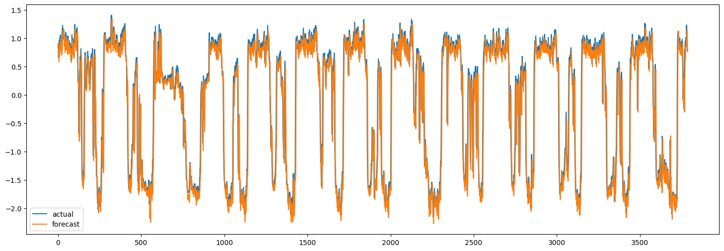
当然,这里的目标是演示方法,而不是达到最佳性能。为了提高模型的准确性,所有模型超参数都应经过仔细调整。此外,可以堆叠多个 LSTMGC 块以增加模型的表示能力。