Keras 调试技巧
作者: fchollet
创建日期 2020/05/16
最后修改日期 2023/11/16
描述:四个简单技巧,帮助您调试 Keras 代码。

简介
通常,您几乎可以用不写代码的方式在 Keras 中完成几乎所有事情:无论是实现一种新的 GAN 类型还是用于图像分割的最新卷积网络架构,您通常都可以坚持调用内置方法。由于所有内置方法都会进行广泛的输入验证检查,因此您几乎不需要进行调试。完全由内置层组成的 Functional API 模型将一次性运行——如果您能编译它,它就能运行。
但是,有时您需要深入研究并编写自己的代码。以下是一些常见示例:
- 创建新的
Layer子类。 - 创建自定义
Metric子类。 - 在
Model上实现自定义train_step。
本文档提供了一些简单的技巧,以帮助您在这些情况下进行调试。
技巧 1:在测试整体之前先测试每个部分
如果您创建了任何可能无法按预期工作的对象,请不要直接将其放入端到端流程中然后看着火花四溅。相反,先在隔离环境中测试您的自定义对象。这似乎很明显——但您会惊讶于人们有多么经常不从这一点开始。
- 如果您编写了自定义层,请不要立即在整个模型上调用
fit()。先在一些测试数据上调用您的层。 - 如果您编写了自定义指标,请先为其一些参考输入打印其输出。
这是一个简单的示例。让我们编写一个带有错误的自定义层
import os

# The last example uses tf.GradientTape and thus requires TensorFlow.
# However, all tips here are applicable with all backends.
os.environ["KERAS_BACKEND"] = "tensorflow"

import keras
from keras import layers
from keras import ops
import numpy as np
import tensorflow as tf


class MyAntirectifier(layers.Layer):
    def build(self, input_shape):
        output_dim = input_shape[-1]
        self.kernel = self.add_weight(
            shape=(output_dim * 2, output_dim),
            initializer="he_normal",
            name="kernel",
            trainable=True,
        )

    def call(self, inputs):
        # Take the positive part of the input
        pos = ops.relu(inputs)
        # Take the negative part of the input
        neg = ops.relu(-inputs)
        # Concatenate the positive and negative parts
        concatenated = ops.concatenate([pos, neg], axis=0)
        # Project the concatenation down to the same dimensionality as the input
        return ops.matmul(concatenated, self.kernel)
现在,与其直接在端到端模型中使用它,不如让我们尝试在一些测试数据上调用该层
x = tf.random.normal(shape=(2, 5))
y = MyAntirectifier()(x)
我们收到以下错误
...
      1 x = tf.random.normal(shape=(2, 5))
----> 2 y = MyAntirectifier()(x)
...
     17         neg = tf.nn.relu(-inputs)
     18         concatenated = tf.concat([pos, neg], axis=0)
---> 19         return tf.matmul(concatenated, self.kernel)
...
InvalidArgumentError: Matrix size-incompatible: In[0]: [4,5], In[1]: [10,5] [Op:MatMul]
看起来我们 matmul 操作中的输入张量形状可能不正确。让我们添加一个打印语句来检查实际形状
class MyAntirectifier(layers.Layer):
    def build(self, input_shape):
        output_dim = input_shape[-1]
        self.kernel = self.add_weight(
            shape=(output_dim * 2, output_dim),
            initializer="he_normal",
            name="kernel",
            trainable=True,
        )

    def call(self, inputs):
        pos = ops.relu(inputs)
        neg = ops.relu(-inputs)
        print("pos.shape:", pos.shape)
        print("neg.shape:", neg.shape)
        concatenated = ops.concatenate([pos, neg], axis=0)
        print("concatenated.shape:", concatenated.shape)
        print("kernel.shape:", self.kernel.shape)
        return ops.matmul(concatenated, self.kernel)
我们得到以下结果
pos.shape: (2, 5)
neg.shape: (2, 5)
concatenated.shape: (4, 5)
kernel.shape: (10, 5)
原来我们对 concat 操作使用了错误的轴!我们应该沿着特征轴 1 连接 neg 和 pos,而不是批次轴 0。这是正确的版本
class MyAntirectifier(layers.Layer):
    def build(self, input_shape):
        output_dim = input_shape[-1]
        self.kernel = self.add_weight(
            shape=(output_dim * 2, output_dim),
            initializer="he_normal",
            name="kernel",
            trainable=True,
        )

    def call(self, inputs):
        pos = ops.relu(inputs)
        neg = ops.relu(-inputs)
        print("pos.shape:", pos.shape)
        print("neg.shape:", neg.shape)
        concatenated = ops.concatenate([pos, neg], axis=1)
        print("concatenated.shape:", concatenated.shape)
        print("kernel.shape:", self.kernel.shape)
        return ops.matmul(concatenated, self.kernel)
现在我们的代码可以正常工作了
x = keras.random.normal(shape=(2, 5))
y = MyAntirectifier()(x)
pos.shape: (2, 5)
neg.shape: (2, 5)
concatenated.shape: (2, 10)
kernel.shape: (10, 5)
技巧 2:使用 model.summary() 和 plot_model() 检查层输出形状
如果您正在处理复杂的网络拓扑,您将需要一种方法来可视化您的层是如何连接的以及它们如何转换通过它们的数据。
这是一个示例。考虑这个具有三个输入和两个输出的模型(摘自 Functional API 指南)
num_tags = 12  # Number of unique issue tags
num_words = 10000  # Size of vocabulary obtained when preprocessing text data
num_departments = 4  # Number of departments for predictions

title_input = keras.Input(
    shape=(None,), name="title"
)  # Variable-length sequence of ints
body_input = keras.Input(shape=(None,), name="body")  # Variable-length sequence of ints
tags_input = keras.Input(
    shape=(num_tags,), name="tags"
)  # Binary vectors of size `num_tags`

# Embed each word in the title into a 64-dimensional vector
title_features = layers.Embedding(num_words, 64)(title_input)
# Embed each word in the text into a 64-dimensional vector
body_features = layers.Embedding(num_words, 64)(body_input)

# Reduce sequence of embedded words in the title into a single 128-dimensional vector
title_features = layers.LSTM(128)(title_features)
# Reduce sequence of embedded words in the body into a single 32-dimensional vector
body_features = layers.LSTM(32)(body_features)

# Merge all available features into a single large vector via concatenation
x = layers.concatenate([title_features, body_features, tags_input])

# Stick a logistic regression for priority prediction on top of the features
priority_pred = layers.Dense(1, name="priority")(x)
# Stick a department classifier on top of the features
department_pred = layers.Dense(num_departments, name="department")(x)

# Instantiate an end-to-end model predicting both priority and department
model = keras.Model(
    inputs=[title_input, body_input, tags_input],
    outputs=[priority_pred, department_pred],
)
调用 summary() 可以帮助您检查每个层的输出形状
model.summary()
Model: "functional_1"
┏━━━━━━━━━━━━━━━━━━━━━┳━━━━━━━━━━━━━━━━━━━┳━━━━━━━━━┳━━━━━━━━━━━━━━━━━━━━━━┓
┃ Layer (type)        ┃ Output Shape      ┃ Param # ┃ Connected to         ┃
┡━━━━━━━━━━━━━━━━━━━━━╇━━━━━━━━━━━━━━━━━━━╇━━━━━━━━━╇━━━━━━━━━━━━━━━━━━━━━━┩
│ title (InputLayer)  │ (None, None)      │       0 │ -                    │
├─────────────────────┼───────────────────┼─────────┼──────────────────────┤
│ body (InputLayer)   │ (None, None)      │       0 │ -                    │
├─────────────────────┼───────────────────┼─────────┼──────────────────────┤
│ embedding           │ (None, None, 64)  │ 640,000 │ title[0][0]          │
│ (Embedding)         │                   │         │                      │
├─────────────────────┼───────────────────┼─────────┼──────────────────────┤
│ embedding_1         │ (None, None, 64)  │ 640,000 │ body[0][0]           │
│ (Embedding)         │                   │         │                      │
├─────────────────────┼───────────────────┼─────────┼──────────────────────┤
│ lstm (LSTM)         │ (None, 128)       │  98,816 │ embedding[0][0]      │
├─────────────────────┼───────────────────┼─────────┼──────────────────────┤
│ lstm_1 (LSTM)       │ (None, 32)        │  12,416 │ embedding_1[0][0]    │
├─────────────────────┼───────────────────┼─────────┼──────────────────────┤
│ tags (InputLayer)   │ (None, 12)        │       0 │ -                    │
├─────────────────────┼───────────────────┼─────────┼──────────────────────┤
│ concatenate         │ (None, 172)       │       0 │ lstm[0][0],          │
│ (Concatenate)       │                   │         │ lstm_1[0][0],        │
│                     │                   │         │ tags[0][0]           │
├─────────────────────┼───────────────────┼─────────┼──────────────────────┤
│ priority (Dense)    │ (None, 1)         │     173 │ concatenate[0][0]    │
├─────────────────────┼───────────────────┼─────────┼──────────────────────┤
│ department (Dense)  │ (None, 4)         │     692 │ concatenate[0][0]    │
└─────────────────────┴───────────────────┴─────────┴──────────────────────┘
Total params: 1,392,097 (5.31 MB)
Trainable params: 1,392,097 (5.31 MB)
Non-trainable params: 0 (0.00 B)
您还可以使用 plot_model 来可视化整个网络拓扑以及输出形状
keras.utils.plot_model(model, show_shapes=True)
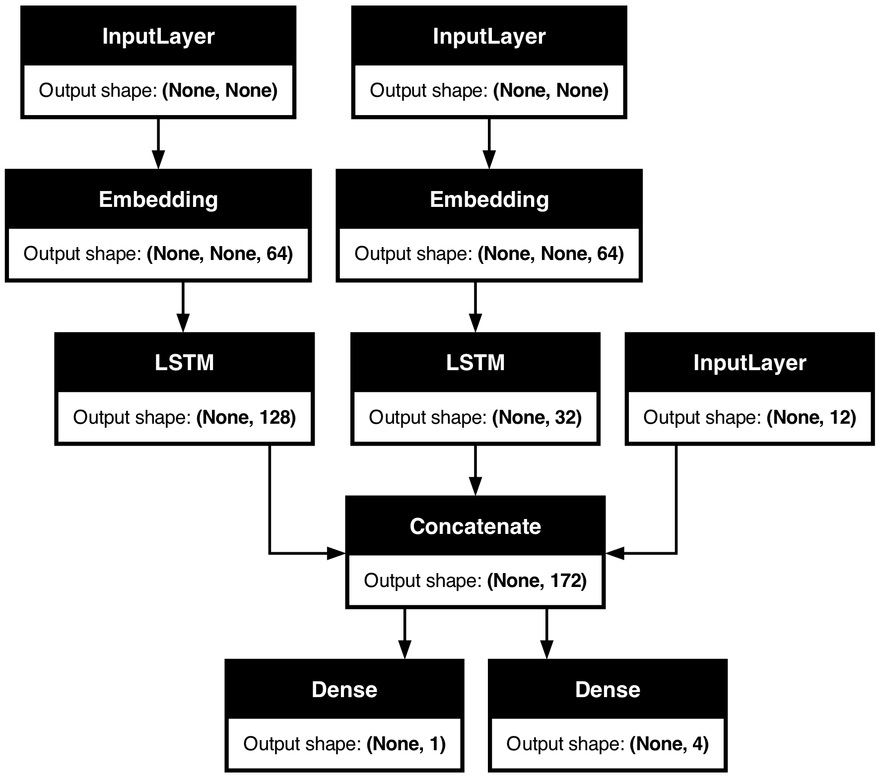
有了这个图,任何连接级别的错误都会立即显现出来。
技巧 3:要调试 fit() 过程中发生的事情,请使用 run_eagerly=True
fit() 方法速度很快:它运行一个经过高度优化、完全编译的计算图。这对性能很好,但这也意味着您正在执行的代码不是您编写的 Python 代码。这在调试时可能会有问题。正如您可能还记得的,Python 很慢——所以我们将其用作暂存语言,而不是执行语言。
幸运的是,有一个简单的方法可以“调试模式”下完全以惰性模式运行您的代码:将 run_eagerly=True 传递给 compile()。您的 fit() 调用现在将逐行执行,无需任何优化。它速度较慢,但可以打印中间张量的值,或使用 Python 调试器。非常适合调试。
这是一个基本示例:让我们编写一个非常简单的模型,其中包含自定义的 train_step() 方法。我们的模型只是实现了梯度下降,但它使用的是一阶和二阶梯度组合,而不是一阶梯度。到目前为止还很简单。
您能发现我们哪里做错了什么吗?
class MyModel(keras.Model):
    def train_step(self, data):
        inputs, targets = data
        trainable_vars = self.trainable_variables
        with tf.GradientTape() as tape2:
            with tf.GradientTape() as tape1:
                y_pred = self(inputs, training=True)  # Forward pass
                # Compute the loss value
                # (the loss function is configured in `compile()`)
                loss = self.compute_loss(y=targets, y_pred=y_pred)
            # Compute first-order gradients
            dl_dw = tape1.gradient(loss, trainable_vars)
        # Compute second-order gradients
        d2l_dw2 = tape2.gradient(dl_dw, trainable_vars)

        # Combine first-order and second-order gradients
        grads = [0.5 * w1 + 0.5 * w2 for (w1, w2) in zip(d2l_dw2, dl_dw)]

        # Update weights
        self.optimizer.apply_gradients(zip(grads, trainable_vars))

        # Update metrics (includes the metric that tracks the loss)
        for metric in self.metrics:
            if metric.name == "loss":
                metric.update_state(loss)
            else:
                metric.update_state(targets, y_pred)

        # Return a dict mapping metric names to current value
        return {m.name: m.result() for m in self.metrics}
让我们用这个自定义损失函数在 MNIST 上训练一个单层模型。
我们选择(有些随机)批次大小为 1024,学习率为 0.1。其基本思想是使用比通常更大的批次和更大的学习率,因为我们“改进”的梯度应该会让我们更快地收敛。
# Construct an instance of MyModel
def get_model():
    inputs = keras.Input(shape=(784,))
    intermediate = layers.Dense(256, activation="relu")(inputs)
    outputs = layers.Dense(10, activation="softmax")(intermediate)
    model = MyModel(inputs, outputs)
    return model


# Prepare data
(x_train, y_train), _ = keras.datasets.mnist.load_data()
x_train = np.reshape(x_train, (-1, 784)) / 255

model = get_model()
model.compile(
    optimizer=keras.optimizers.SGD(learning_rate=1e-2),
    loss="sparse_categorical_crossentropy",
)
model.fit(x_train, y_train, epochs=3, batch_size=1024, validation_split=0.1)
Epoch 1/3
 53/53 ━━━━━━━━━━━━━━━━━━━━ 0s 7ms/step - loss: 2.4264 - val_loss: 2.3036
Epoch 2/3
 53/53 ━━━━━━━━━━━━━━━━━━━━ 0s 6ms/step - loss: 2.3111 - val_loss: 2.3387
Epoch 3/3
 53/53 ━━━━━━━━━━━━━━━━━━━━ 0s 7ms/step - loss: 2.3442 - val_loss: 2.3697

<keras.src.callbacks.history.History at 0x29a899600>
哦不,它没有收敛!有什么东西没有按计划进行。
是时候逐步打印我们梯度的情况了。
我们在 train_step 方法中添加了各种 print 语句,并确保将 run_eagerly=True 传递给 compile() 以逐步、惰性地运行我们的代码。
class MyModel(keras.Model):
    def train_step(self, data):
        print()
        print("----Start of step: %d" % (self.step_counter,))
        self.step_counter += 1

        inputs, targets = data
        trainable_vars = self.trainable_variables
        with tf.GradientTape() as tape2:
            with tf.GradientTape() as tape1:
                y_pred = self(inputs, training=True)  # Forward pass
                # Compute the loss value
                # (the loss function is configured in `compile()`)
                loss = self.compute_loss(y=targets, y_pred=y_pred)
            # Compute first-order gradients
            dl_dw = tape1.gradient(loss, trainable_vars)
        # Compute second-order gradients
        d2l_dw2 = tape2.gradient(dl_dw, trainable_vars)

        print("Max of dl_dw[0]: %.4f" % tf.reduce_max(dl_dw[0]))
        print("Min of dl_dw[0]: %.4f" % tf.reduce_min(dl_dw[0]))
        print("Mean of dl_dw[0]: %.4f" % tf.reduce_mean(dl_dw[0]))
        print("-")
        print("Max of d2l_dw2[0]: %.4f" % tf.reduce_max(d2l_dw2[0]))
        print("Min of d2l_dw2[0]: %.4f" % tf.reduce_min(d2l_dw2[0]))
        print("Mean of d2l_dw2[0]: %.4f" % tf.reduce_mean(d2l_dw2[0]))

        # Combine first-order and second-order gradients
        grads = [0.5 * w1 + 0.5 * w2 for (w1, w2) in zip(d2l_dw2, dl_dw)]

        # Update weights
        self.optimizer.apply_gradients(zip(grads, trainable_vars))

        # Update metrics (includes the metric that tracks the loss)
        for metric in self.metrics:
            if metric.name == "loss":
                metric.update_state(loss)
            else:
                metric.update_state(targets, y_pred)

        # Return a dict mapping metric names to current value
        return {m.name: m.result() for m in self.metrics}


model = get_model()
model.compile(
    optimizer=keras.optimizers.SGD(learning_rate=1e-2),
    loss="sparse_categorical_crossentropy",
    metrics=["sparse_categorical_accuracy"],
    run_eagerly=True,
)
model.step_counter = 0
# We pass epochs=1 and steps_per_epoch=10 to only run 10 steps of training.
model.fit(x_train, y_train, epochs=1, batch_size=1024, verbose=0, steps_per_epoch=10)
----Start of step: 0
Max of dl_dw[0]: 0.0332
Min of dl_dw[0]: -0.0288
Mean of dl_dw[0]: 0.0003
-
Max of d2l_dw2[0]: 5.2691
Min of d2l_dw2[0]: -2.6968
Mean of d2l_dw2[0]: 0.0981
----Start of step: 1
Max of dl_dw[0]: 0.0445
Min of dl_dw[0]: -0.0169
Mean of dl_dw[0]: 0.0013
-
Max of d2l_dw2[0]: 3.3575
Min of d2l_dw2[0]: -1.9024
Mean of d2l_dw2[0]: 0.0726
----Start of step: 2
Max of dl_dw[0]: 0.0669
Min of dl_dw[0]: -0.0153
Mean of dl_dw[0]: 0.0013
-
Max of d2l_dw2[0]: 5.0661
Min of d2l_dw2[0]: -1.7168
Mean of d2l_dw2[0]: 0.0809
----Start of step: 3
Max of dl_dw[0]: 0.0545
Min of dl_dw[0]: -0.0125
Mean of dl_dw[0]: 0.0008
-
Max of d2l_dw2[0]: 6.5223
Min of d2l_dw2[0]: -0.6604
Mean of d2l_dw2[0]: 0.0991
----Start of step: 4
Max of dl_dw[0]: 0.0247
Min of dl_dw[0]: -0.0152
Mean of dl_dw[0]: -0.0001
-
Max of d2l_dw2[0]: 2.8030
Min of d2l_dw2[0]: -0.1156
Mean of d2l_dw2[0]: 0.0321
----Start of step: 5
Max of dl_dw[0]: 0.0051
Min of dl_dw[0]: -0.0096
Mean of dl_dw[0]: -0.0001
-
Max of d2l_dw2[0]: 0.2545
Min of d2l_dw2[0]: -0.0284
Mean of d2l_dw2[0]: 0.0079
----Start of step: 6
Max of dl_dw[0]: 0.0041
Min of dl_dw[0]: -0.0102
Mean of dl_dw[0]: -0.0001
-
Max of d2l_dw2[0]: 0.2198
Min of d2l_dw2[0]: -0.0175
Mean of d2l_dw2[0]: 0.0069
----Start of step: 7
Max of dl_dw[0]: 0.0035
Min of dl_dw[0]: -0.0086
Mean of dl_dw[0]: -0.0001
-
Max of d2l_dw2[0]: 0.1485
Min of d2l_dw2[0]: -0.0175
Mean of d2l_dw2[0]: 0.0060
----Start of step: 8
Max of dl_dw[0]: 0.0039
Min of dl_dw[0]: -0.0094
Mean of dl_dw[0]: -0.0001
-
Max of d2l_dw2[0]: 0.1454
Min of d2l_dw2[0]: -0.0130
Mean of d2l_dw2[0]: 0.0061
----Start of step: 9
Max of dl_dw[0]: 0.0028
Min of dl_dw[0]: -0.0087
Mean of dl_dw[0]: -0.0001
-
Max of d2l_dw2[0]: 0.1491
Min of d2l_dw2[0]: -0.0326
Mean of d2l_dw2[0]: 0.0058

<keras.src.callbacks.history.History at 0x2a0d1e440>
我们学到了什么?
- 一阶和二阶梯度可能具有数量级上的差异。
- 有时,它们甚至可能没有相同的符号。
- 它们的值在每一步都可能差异很大。
这让我们产生了一个显而易见的想法:在组合梯度之前对它们进行归一化。
class MyModel(keras.Model):
    def train_step(self, data):
        inputs, targets = data
        trainable_vars = self.trainable_variables
        with tf.GradientTape() as tape2:
            with tf.GradientTape() as tape1:
                y_pred = self(inputs, training=True)  # Forward pass
                # Compute the loss value
                # (the loss function is configured in `compile()`)
                loss = self.compute_loss(y=targets, y_pred=y_pred)
            # Compute first-order gradients
            dl_dw = tape1.gradient(loss, trainable_vars)
        # Compute second-order gradients
        d2l_dw2 = tape2.gradient(dl_dw, trainable_vars)

        dl_dw = [tf.math.l2_normalize(w) for w in dl_dw]
        d2l_dw2 = [tf.math.l2_normalize(w) for w in d2l_dw2]

        # Combine first-order and second-order gradients
        grads = [0.5 * w1 + 0.5 * w2 for (w1, w2) in zip(d2l_dw2, dl_dw)]

        # Update weights
        self.optimizer.apply_gradients(zip(grads, trainable_vars))

        # Update metrics (includes the metric that tracks the loss)
        for metric in self.metrics:
            if metric.name == "loss":
                metric.update_state(loss)
            else:
                metric.update_state(targets, y_pred)

        # Return a dict mapping metric names to current value
        return {m.name: m.result() for m in self.metrics}


model = get_model()
model.compile(
    optimizer=keras.optimizers.SGD(learning_rate=1e-2),
    loss="sparse_categorical_crossentropy",
    metrics=["sparse_categorical_accuracy"],
)
model.fit(x_train, y_train, epochs=5, batch_size=1024, validation_split=0.1)
Epoch 1/5
 53/53 ━━━━━━━━━━━━━━━━━━━━ 1s 7ms/step - sparse_categorical_accuracy: 0.1250 - loss: 2.3185 - val_loss: 2.0502 - val_sparse_categorical_accuracy: 0.3373
Epoch 2/5
 53/53 ━━━━━━━━━━━━━━━━━━━━ 0s 6ms/step - sparse_categorical_accuracy: 0.3966 - loss: 1.9934 - val_loss: 1.8032 - val_sparse_categorical_accuracy: 0.5698
Epoch 3/5
 53/53 ━━━━━━━━━━━━━━━━━━━━ 0s 7ms/step - sparse_categorical_accuracy: 0.5663 - loss: 1.7784 - val_loss: 1.6241 - val_sparse_categorical_accuracy: 0.6470
Epoch 4/5
 53/53 ━━━━━━━━━━━━━━━━━━━━ 0s 7ms/step - sparse_categorical_accuracy: 0.6135 - loss: 1.6256 - val_loss: 1.5010 - val_sparse_categorical_accuracy: 0.6595
Epoch 5/5
 53/53 ━━━━━━━━━━━━━━━━━━━━ 0s 7ms/step - sparse_categorical_accuracy: 0.6216 - loss: 1.5173 - val_loss: 1.4169 - val_sparse_categorical_accuracy: 0.6625

<keras.src.callbacks.history.History at 0x2a0d4c640>
现在,训练可以收敛了!它根本不起作用,但至少模型能学到一些东西。
在花费几分钟调整参数后,我们得到了以下配置,该配置效果还算可以(实现了 97% 的验证准确率,并且在过拟合方面似乎相当稳健)
- 使用
0.2 * w1 + 0.8 * w2来组合梯度。 - 使用随时间线性衰减的学习率。
我不会说这个想法是可行的——这根本不是你应该进行二阶优化(提示:参见牛顿和高斯-牛顿方法、拟牛顿方法和 BFGS)。但希望这个演示能让你了解如何通过调试摆脱不舒服的训练情况。
记住:使用 run_eagerly=True 来调试 fit() 中发生的事情。当您的代码终于按预期工作时,请务必移除此标志以获得最佳运行时性能!
这是我们最后的训练运行
class MyModel(keras.Model):
    def train_step(self, data):
        inputs, targets = data
        trainable_vars = self.trainable_variables
        with tf.GradientTape() as tape2:
            with tf.GradientTape() as tape1:
                y_pred = self(inputs, training=True)  # Forward pass
                # Compute the loss value
                # (the loss function is configured in `compile()`)
                loss = self.compute_loss(y=targets, y_pred=y_pred)
            # Compute first-order gradients
            dl_dw = tape1.gradient(loss, trainable_vars)
        # Compute second-order gradients
        d2l_dw2 = tape2.gradient(dl_dw, trainable_vars)

        dl_dw = [tf.math.l2_normalize(w) for w in dl_dw]
        d2l_dw2 = [tf.math.l2_normalize(w) for w in d2l_dw2]

        # Combine first-order and second-order gradients
        grads = [0.2 * w1 + 0.8 * w2 for (w1, w2) in zip(d2l_dw2, dl_dw)]

        # Update weights
        self.optimizer.apply_gradients(zip(grads, trainable_vars))

        # Update metrics (includes the metric that tracks the loss)
        for metric in self.metrics:
            if metric.name == "loss":
                metric.update_state(loss)
            else:
                metric.update_state(targets, y_pred)

        # Return a dict mapping metric names to current value
        return {m.name: m.result() for m in self.metrics}


model = get_model()
lr = learning_rate = keras.optimizers.schedules.InverseTimeDecay(
    initial_learning_rate=0.1, decay_steps=25, decay_rate=0.1
)
model.compile(
    optimizer=keras.optimizers.SGD(lr),
    loss="sparse_categorical_crossentropy",
    metrics=["sparse_categorical_accuracy"],
)
model.fit(x_train, y_train, epochs=50, batch_size=2048, validation_split=0.1)
Epoch 1/50
 27/27 ━━━━━━━━━━━━━━━━━━━━ 1s 14ms/step - sparse_categorical_accuracy: 0.5056 - loss: 1.7508 - val_loss: 0.6378 - val_sparse_categorical_accuracy: 0.8658
Epoch 2/50
 27/27 ━━━━━━━━━━━━━━━━━━━━ 0s 10ms/step - sparse_categorical_accuracy: 0.8407 - loss: 0.6323 - val_loss: 0.4039 - val_sparse_categorical_accuracy: 0.8970
Epoch 3/50
 27/27 ━━━━━━━━━━━━━━━━━━━━ 0s 10ms/step - sparse_categorical_accuracy: 0.8807 - loss: 0.4472 - val_loss: 0.3243 - val_sparse_categorical_accuracy: 0.9120
Epoch 4/50
 27/27 ━━━━━━━━━━━━━━━━━━━━ 0s 10ms/step - sparse_categorical_accuracy: 0.8947 - loss: 0.3781 - val_loss: 0.2861 - val_sparse_categorical_accuracy: 0.9235
Epoch 5/50
 27/27 ━━━━━━━━━━━━━━━━━━━━ 0s 11ms/step - sparse_categorical_accuracy: 0.9022 - loss: 0.3453 - val_loss: 0.2622 - val_sparse_categorical_accuracy: 0.9288
Epoch 6/50
 27/27 ━━━━━━━━━━━━━━━━━━━━ 0s 11ms/step - sparse_categorical_accuracy: 0.9093 - loss: 0.3243 - val_loss: 0.2523 - val_sparse_categorical_accuracy: 0.9303
Epoch 7/50
 27/27 ━━━━━━━━━━━━━━━━━━━━ 0s 11ms/step - sparse_categorical_accuracy: 0.9148 - loss: 0.3021 - val_loss: 0.2362 - val_sparse_categorical_accuracy: 0.9338
Epoch 8/50
 27/27 ━━━━━━━━━━━━━━━━━━━━ 0s 11ms/step - sparse_categorical_accuracy: 0.9184 - loss: 0.2899 - val_loss: 0.2289 - val_sparse_categorical_accuracy: 0.9365
Epoch 9/50
 27/27 ━━━━━━━━━━━━━━━━━━━━ 0s 11ms/step - sparse_categorical_accuracy: 0.9212 - loss: 0.2784 - val_loss: 0.2183 - val_sparse_categorical_accuracy: 0.9383
Epoch 10/50
 27/27 ━━━━━━━━━━━━━━━━━━━━ 0s 11ms/step - sparse_categorical_accuracy: 0.9246 - loss: 0.2670 - val_loss: 0.2097 - val_sparse_categorical_accuracy: 0.9405
Epoch 11/50
 27/27 ━━━━━━━━━━━━━━━━━━━━ 0s 11ms/step - sparse_categorical_accuracy: 0.9267 - loss: 0.2563 - val_loss: 0.2063 - val_sparse_categorical_accuracy: 0.9442
Epoch 12/50
 27/27 ━━━━━━━━━━━━━━━━━━━━ 0s 12ms/step - sparse_categorical_accuracy: 0.9313 - loss: 0.2412 - val_loss: 0.1965 - val_sparse_categorical_accuracy: 0.9458
Epoch 13/50
 27/27 ━━━━━━━━━━━━━━━━━━━━ 0s 12ms/step - sparse_categorical_accuracy: 0.9324 - loss: 0.2411 - val_loss: 0.1917 - val_sparse_categorical_accuracy: 0.9472
Epoch 14/50
 27/27 ━━━━━━━━━━━━━━━━━━━━ 0s 12ms/step - sparse_categorical_accuracy: 0.9359 - loss: 0.2260 - val_loss: 0.1861 - val_sparse_categorical_accuracy: 0.9495
Epoch 15/50
 27/27 ━━━━━━━━━━━━━━━━━━━━ 0s 12ms/step - sparse_categorical_accuracy: 0.9374 - loss: 0.2234 - val_loss: 0.1804 - val_sparse_categorical_accuracy: 0.9517
Epoch 16/50
 27/27 ━━━━━━━━━━━━━━━━━━━━ 0s 14ms/step - sparse_categorical_accuracy: 0.9382 - loss: 0.2196 - val_loss: 0.1761 - val_sparse_categorical_accuracy: 0.9528
Epoch 17/50
 27/27 ━━━━━━━━━━━━━━━━━━━━ 0s 14ms/step - sparse_categorical_accuracy: 0.9417 - loss: 0.2076 - val_loss: 0.1709 - val_sparse_categorical_accuracy: 0.9557
Epoch 18/50
 27/27 ━━━━━━━━━━━━━━━━━━━━ 0s 13ms/step - sparse_categorical_accuracy: 0.9423 - loss: 0.2032 - val_loss: 0.1664 - val_sparse_categorical_accuracy: 0.9555
Epoch 19/50
 27/27 ━━━━━━━━━━━━━━━━━━━━ 0s 12ms/step - sparse_categorical_accuracy: 0.9444 - loss: 0.1953 - val_loss: 0.1616 - val_sparse_categorical_accuracy: 0.9582
Epoch 20/50
 27/27 ━━━━━━━━━━━━━━━━━━━━ 0s 12ms/step - sparse_categorical_accuracy: 0.9451 - loss: 0.1916 - val_loss: 0.1597 - val_sparse_categorical_accuracy: 0.9592
Epoch 21/50
 27/27 ━━━━━━━━━━━━━━━━━━━━ 0s 13ms/step - sparse_categorical_accuracy: 0.9473 - loss: 0.1866 - val_loss: 0.1563 - val_sparse_categorical_accuracy: 0.9615
Epoch 22/50
 27/27 ━━━━━━━━━━━━━━━━━━━━ 0s 12ms/step - sparse_categorical_accuracy: 0.9486 - loss: 0.1818 - val_loss: 0.1520 - val_sparse_categorical_accuracy: 0.9617
Epoch 23/50
 27/27 ━━━━━━━━━━━━━━━━━━━━ 0s 12ms/step - sparse_categorical_accuracy: 0.9502 - loss: 0.1794 - val_loss: 0.1499 - val_sparse_categorical_accuracy: 0.9635
Epoch 24/50
 27/27 ━━━━━━━━━━━━━━━━━━━━ 0s 12ms/step - sparse_categorical_accuracy: 0.9502 - loss: 0.1759 - val_loss: 0.1466 - val_sparse_categorical_accuracy: 0.9640
Epoch 25/50
 27/27 ━━━━━━━━━━━━━━━━━━━━ 0s 12ms/step - sparse_categorical_accuracy: 0.9515 - loss: 0.1714 - val_loss: 0.1437 - val_sparse_categorical_accuracy: 0.9645
Epoch 26/50
 27/27 ━━━━━━━━━━━━━━━━━━━━ 0s 14ms/step - sparse_categorical_accuracy: 0.9535 - loss: 0.1649 - val_loss: 0.1435 - val_sparse_categorical_accuracy: 0.9640
Epoch 27/50
 27/27 ━━━━━━━━━━━━━━━━━━━━ 0s 13ms/step - sparse_categorical_accuracy: 0.9548 - loss: 0.1628 - val_loss: 0.1411 - val_sparse_categorical_accuracy: 0.9650
Epoch 28/50
 27/27 ━━━━━━━━━━━━━━━━━━━━ 0s 12ms/step - sparse_categorical_accuracy: 0.9541 - loss: 0.1620 - val_loss: 0.1384 - val_sparse_categorical_accuracy: 0.9655
Epoch 29/50
 27/27 ━━━━━━━━━━━━━━━━━━━━ 0s 12ms/step - sparse_categorical_accuracy: 0.9564 - loss: 0.1560 - val_loss: 0.1359 - val_sparse_categorical_accuracy: 0.9668
Epoch 30/50
 27/27 ━━━━━━━━━━━━━━━━━━━━ 0s 12ms/step - sparse_categorical_accuracy: 0.9577 - loss: 0.1547 - val_loss: 0.1338 - val_sparse_categorical_accuracy: 0.9672
Epoch 31/50
 27/27 ━━━━━━━━━━━━━━━━━━━━ 0s 12ms/step - sparse_categorical_accuracy: 0.9569 - loss: 0.1520 - val_loss: 0.1329 - val_sparse_categorical_accuracy: 0.9663
Epoch 32/50
 27/27 ━━━━━━━━━━━━━━━━━━━━ 0s 12ms/step - sparse_categorical_accuracy: 0.9582 - loss: 0.1478 - val_loss: 0.1320 - val_sparse_categorical_accuracy: 0.9675
Epoch 33/50
 27/27 ━━━━━━━━━━━━━━━━━━━━ 0s 12ms/step - sparse_categorical_accuracy: 0.9582 - loss: 0.1483 - val_loss: 0.1292 - val_sparse_categorical_accuracy: 0.9670
Epoch 34/50
 27/27 ━━━━━━━━━━━━━━━━━━━━ 0s 12ms/step - sparse_categorical_accuracy: 0.9594 - loss: 0.1448 - val_loss: 0.1274 - val_sparse_categorical_accuracy: 0.9677
Epoch 35/50
 27/27 ━━━━━━━━━━━━━━━━━━━━ 0s 12ms/step - sparse_categorical_accuracy: 0.9587 - loss: 0.1452 - val_loss: 0.1262 - val_sparse_categorical_accuracy: 0.9678
Epoch 36/50
 27/27 ━━━━━━━━━━━━━━━━━━━━ 0s 12ms/step - sparse_categorical_accuracy: 0.9603 - loss: 0.1418 - val_loss: 0.1251 - val_sparse_categorical_accuracy: 0.9677
Epoch 37/50
 27/27 ━━━━━━━━━━━━━━━━━━━━ 0s 12ms/step - sparse_categorical_accuracy: 0.9603 - loss: 0.1402 - val_loss: 0.1238 - val_sparse_categorical_accuracy: 0.9682
Epoch 38/50
 27/27 ━━━━━━━━━━━━━━━━━━━━ 0s 11ms/step - sparse_categorical_accuracy: 0.9618 - loss: 0.1382 - val_loss: 0.1228 - val_sparse_categorical_accuracy: 0.9680
Epoch 39/50
 27/27 ━━━━━━━━━━━━━━━━━━━━ 0s 12ms/step - sparse_categorical_accuracy: 0.9630 - loss: 0.1335 - val_loss: 0.1213 - val_sparse_categorical_accuracy: 0.9695
Epoch 40/50
 27/27 ━━━━━━━━━━━━━━━━━━━━ 0s 12ms/step - sparse_categorical_accuracy: 0.9629 - loss: 0.1327 - val_loss: 0.1198 - val_sparse_categorical_accuracy: 0.9698
Epoch 41/50
 27/27 ━━━━━━━━━━━━━━━━━━━━ 0s 12ms/step - sparse_categorical_accuracy: 0.9639 - loss: 0.1323 - val_loss: 0.1191 - val_sparse_categorical_accuracy: 0.9695
Epoch 42/50
 27/27 ━━━━━━━━━━━━━━━━━━━━ 0s 12ms/step - sparse_categorical_accuracy: 0.9629 - loss: 0.1346 - val_loss: 0.1183 - val_sparse_categorical_accuracy: 0.9692
Epoch 43/50
 27/27 ━━━━━━━━━━━━━━━━━━━━ 0s 12ms/step - sparse_categorical_accuracy: 0.9661 - loss: 0.1262 - val_loss: 0.1182 - val_sparse_categorical_accuracy: 0.9700
Epoch 44/50
 27/27 ━━━━━━━━━━━━━━━━━━━━ 0s 12ms/step - sparse_categorical_accuracy: 0.9652 - loss: 0.1274 - val_loss: 0.1163 - val_sparse_categorical_accuracy: 0.9702
Epoch 45/50
 27/27 ━━━━━━━━━━━━━━━━━━━━ 0s 12ms/step - sparse_categorical_accuracy: 0.9650 - loss: 0.1259 - val_loss: 0.1154 - val_sparse_categorical_accuracy: 0.9708
Epoch 46/50
 27/27 ━━━━━━━━━━━━━━━━━━━━ 0s 11ms/step - sparse_categorical_accuracy: 0.9647 - loss: 0.1246 - val_loss: 0.1148 - val_sparse_categorical_accuracy: 0.9703
Epoch 47/50
 27/27 ━━━━━━━━━━━━━━━━━━━━ 0s 12ms/step - sparse_categorical_accuracy: 0.9659 - loss: 0.1236 - val_loss: 0.1137 - val_sparse_categorical_accuracy: 0.9707
Epoch 48/50
 27/27 ━━━━━━━━━━━━━━━━━━━━ 0s 12ms/step - sparse_categorical_accuracy: 0.9665 - loss: 0.1221 - val_loss: 0.1133 - val_sparse_categorical_accuracy: 0.9710
Epoch 49/50
 27/27 ━━━━━━━━━━━━━━━━━━━━ 0s 12ms/step - sparse_categorical_accuracy: 0.9675 - loss: 0.1192 - val_loss: 0.1124 - val_sparse_categorical_accuracy: 0.9712
Epoch 50/50
 27/27 ━━━━━━━━━━━━━━━━━━━━ 0s 12ms/step - sparse_categorical_accuracy: 0.9664 - loss: 0.1214 - val_loss: 0.1112 - val_sparse_categorical_accuracy: 0.9707

<keras.src.callbacks.history.History at 0x29e76ae60>