用于分子属性预测的消息传递神经网络 (MPNN)
作者: akensert
创建日期 2021/08/16
最后修改日期 2021/12/27
描述: MPNN 实现,用于预测血脑屏障通透性。

简介
在本教程中,我们将实现一种称为“消息传递神经网络”(MPNN)的图神经网络(GNN),用于预测图属性。具体来说,我们将实现一个 MPNN 来预测一种称为血脑屏障通透性(BBBP)的分子属性。
动机:由于分子自然表示为无向图 G = (V, E),其中 V 是顶点(节点;原子)集合,E 是边(键)集合,因此 GNN(如 MPNN)被证明是预测分子属性的有用方法。
到目前为止,随机森林、支持向量机等传统方法常用于预测分子属性。与 GNN 不同,这些传统方法通常基于预先计算的分子特征,如分子量、极性、电荷、碳原子数等。尽管这些分子特征被证明是各种分子属性的良好预测因子,但有人假设,使用这些更“原始”、“低级”的特征可能会带来更好的效果。
参考文献
近年来,人们在开发用于图数据(包括分子图)的神经网络方面付出了很多努力。有关图神经网络的摘要,请参阅例如 A Comprehensive Survey on Graph Neural Networks 和 Graph Neural Networks: A Review of Methods and Applications;有关本教程中实现的特定图神经网络的进一步阅读,请参阅 Neural Message Passing for Quantum Chemistry 和 DeepChem's MPNNModel。
设置
安装 RDKit 和其他依赖项
(以下文本摘自 本教程)。
RDKit 是一个用 C++ 和 Python 编写的计算化学和机器学习软件集合。在本教程中,RDKit 用于方便高效地将 SMILES 转换为分子对象,然后从分子对象中获取原子和键的集合。
SMILES 以 ASCII 字符串的形式表示给定分子的结构。SMILES 字符串是一种紧凑的编码,对于较小的分子来说,它相对易于人类阅读。将分子编码为字符串既减轻了数据库和/或网络搜索给定分子的负担,又促进了这些操作。RDKit 使用算法将给定的 SMILES 精确转换为分子对象,然后可以使用该对象计算大量分子属性/特征。
请注意,RDKit 通常通过 Conda 安装。但是,感谢 rdkit_platform_wheels,现在(为了本教程的目的)可以通过 pip 轻松安装 RDKit,如下所示:
pip -q install rdkit-pypi
为了方便高效地读取 csv 文件和可视化,需要安装以下内容:
pip -q install pandas
pip -q install Pillow
pip -q install matplotlib
pip -q install pydot
sudo apt-get -qq install graphviz
导入包
import os

# Temporary suppress tf logs
os.environ["TF_CPP_MIN_LOG_LEVEL"] = "3"

import tensorflow as tf
from tensorflow import keras
from tensorflow.keras import layers
import numpy as np
import pandas as pd
import matplotlib.pyplot as plt
import warnings
from rdkit import Chem
from rdkit import RDLogger
from rdkit.Chem.Draw import IPythonConsole
from rdkit.Chem.Draw import MolsToGridImage

# Temporary suppress warnings and RDKit logs
warnings.filterwarnings("ignore")
RDLogger.DisableLog("rdApp.*")

np.random.seed(42)
tf.random.set_seed(42)
数据集
有关该数据集的信息可以在 A Bayesian Approach to in Silico Blood-Brain Barrier Penetration Modeling 和 MoleculeNet: A Benchmark for Molecular Machine Learning 中找到。数据集将从 MoleculeNet.org 下载。
关于
数据集包含 **2,050** 个分子。每个分子都带有 **名称**、**标签**和 **SMILES** 字符串。
血脑屏障(BBB)是分隔血液和脑细胞外液的屏障,因此会阻止大多数药物(分子)进入大脑。因此,BBBP 的研究对于开发旨在靶向中枢神经系统的新药至关重要。此数据集的标签是二元的(1 或 0),表示分子的通透性。
csv_path = keras.utils.get_file(
    "BBBP.csv", "https://deepchemdata.s3-us-west-1.amazonaws.com/datasets/BBBP.csv"
)

df = pd.read_csv(csv_path, usecols=[1, 2, 3])
df.iloc[96:104]
| 名称 | p_np | smiles | |
|---|---|---|---|
| 96 | cefoxitin | 1 | CO[C@]1(NC(=O)Cc2sccc2)[C@H]3SCC(=C(N3C1=O)C(O... |
| 97 | Org34167 | 1 | NC(CC=C)c1ccccc1c2noc3c2cccc3 |
| 98 | 9-OH Risperidone | 1 | OC1C(N2CCC1)=NC(C)=C(CCN3CCC(CC3)c4c5ccc(F)cc5... |
| 99 | acetaminophen | 1 | CC(=O)Nc1ccc(O)cc1 |
| 100 | acetylsalicylate | 0 | CC(=O)Oc1ccccc1C(O)=O |
| 101 | allopurinol | 0 | O=C1N=CN=C2NNC=C12 |
| 102 | Alprostadil | 0 | CCCCC[C@H](O)/C=C/[C@H]1[C@H](O)CC(=O)[C@@H]1C... |
| 103 | aminophylline | 0 | CN1C(=O)N(C)c2nc[nH]c2C1=O.CN3C(=O)N(C)c4nc[nH... |
定义特征
为了对原子和键(我们稍后需要)进行特征编码,我们将定义两个类:分别为 AtomFeaturizer 和 BondFeaturizer。
为了减少代码行数,即为了使本教程简短明了,只考虑少数(原子和键)特征:[原子特征] 符号(元素)、价电子数、氢键数、轨道杂化,[键特征] (共价)键类型 和 共轭。
class Featurizer:
    def __init__(self, allowable_sets):
        self.dim = 0
        self.features_mapping = {}
        for k, s in allowable_sets.items():
            s = sorted(list(s))
            self.features_mapping[k] = dict(zip(s, range(self.dim, len(s) + self.dim)))
            self.dim += len(s)

    def encode(self, inputs):
        output = np.zeros((self.dim,))
        for name_feature, feature_mapping in self.features_mapping.items():
            feature = getattr(self, name_feature)(inputs)
            if feature not in feature_mapping:
                continue
            output[feature_mapping[feature]] = 1.0
        return output


class AtomFeaturizer(Featurizer):
    def __init__(self, allowable_sets):
        super().__init__(allowable_sets)

    def symbol(self, atom):
        return atom.GetSymbol()

    def n_valence(self, atom):
        return atom.GetTotalValence()

    def n_hydrogens(self, atom):
        return atom.GetTotalNumHs()

    def hybridization(self, atom):
        return atom.GetHybridization().name.lower()


class BondFeaturizer(Featurizer):
    def __init__(self, allowable_sets):
        super().__init__(allowable_sets)
        self.dim += 1

    def encode(self, bond):
        output = np.zeros((self.dim,))
        if bond is None:
            output[-1] = 1.0
            return output
        output = super().encode(bond)
        return output

    def bond_type(self, bond):
        return bond.GetBondType().name.lower()

    def conjugated(self, bond):
        return bond.GetIsConjugated()


atom_featurizer = AtomFeaturizer(
    allowable_sets={
        "symbol": {"B", "Br", "C", "Ca", "Cl", "F", "H", "I", "N", "Na", "O", "P", "S"},
        "n_valence": {0, 1, 2, 3, 4, 5, 6},
        "n_hydrogens": {0, 1, 2, 3, 4},
        "hybridization": {"s", "sp", "sp2", "sp3"},
    }
)

bond_featurizer = BondFeaturizer(
    allowable_sets={
        "bond_type": {"single", "double", "triple", "aromatic"},
        "conjugated": {True, False},
    }
)
生成图
在我们可以从 SMILES 生成完整的图之前,我们需要实现以下函数:
-
molecule_from_smiles,它接收 SMILES 作为输入并返回分子对象。这全部由 RDKit 处理。 -
graph_from_molecule,它接收分子对象作为输入并返回一个图,表示为三元组(原子特征、键特征、对索引)。为此,我们将利用之前定义的类。
最后,我们现在可以实现函数 graphs_from_smiles,该函数将函数(1)和随后的(2)应用于训练、验证和测试数据集的所有 SMILES。
注意:尽管建议对此数据集进行支架拆分(参见 此处),但为简单起见,执行了简单的随机拆分。
def molecule_from_smiles(smiles):
    # MolFromSmiles(m, sanitize=True) should be equivalent to
    # MolFromSmiles(m, sanitize=False) -> SanitizeMol(m) -> AssignStereochemistry(m, ...)
    molecule = Chem.MolFromSmiles(smiles, sanitize=False)

    # If sanitization is unsuccessful, catch the error, and try again without
    # the sanitization step that caused the error
    flag = Chem.SanitizeMol(molecule, catchErrors=True)
    if flag != Chem.SanitizeFlags.SANITIZE_NONE:
        Chem.SanitizeMol(molecule, sanitizeOps=Chem.SanitizeFlags.SANITIZE_ALL ^ flag)

    Chem.AssignStereochemistry(molecule, cleanIt=True, force=True)
    return molecule


def graph_from_molecule(molecule):
    # Initialize graph
    atom_features = []
    bond_features = []
    pair_indices = []

    for atom in molecule.GetAtoms():
        atom_features.append(atom_featurizer.encode(atom))

        # Add self-loops
        pair_indices.append([atom.GetIdx(), atom.GetIdx()])
        bond_features.append(bond_featurizer.encode(None))

        for neighbor in atom.GetNeighbors():
            bond = molecule.GetBondBetweenAtoms(atom.GetIdx(), neighbor.GetIdx())
            pair_indices.append([atom.GetIdx(), neighbor.GetIdx()])
            bond_features.append(bond_featurizer.encode(bond))

    return np.array(atom_features), np.array(bond_features), np.array(pair_indices)


def graphs_from_smiles(smiles_list):
    # Initialize graphs
    atom_features_list = []
    bond_features_list = []
    pair_indices_list = []

    for smiles in smiles_list:
        molecule = molecule_from_smiles(smiles)
        atom_features, bond_features, pair_indices = graph_from_molecule(molecule)

        atom_features_list.append(atom_features)
        bond_features_list.append(bond_features)
        pair_indices_list.append(pair_indices)

    # Convert lists to ragged tensors for tf.data.Dataset later on
    return (
        tf.ragged.constant(atom_features_list, dtype=tf.float32),
        tf.ragged.constant(bond_features_list, dtype=tf.float32),
        tf.ragged.constant(pair_indices_list, dtype=tf.int64),
    )


# Shuffle array of indices ranging from 0 to 2049
permuted_indices = np.random.permutation(np.arange(df.shape[0]))

# Train set: 80 % of data
train_index = permuted_indices[: int(df.shape[0] * 0.8)]
x_train = graphs_from_smiles(df.iloc[train_index].smiles)
y_train = df.iloc[train_index].p_np

# Valid set: 19 % of data
valid_index = permuted_indices[int(df.shape[0] * 0.8) : int(df.shape[0] * 0.99)]
x_valid = graphs_from_smiles(df.iloc[valid_index].smiles)
y_valid = df.iloc[valid_index].p_np

# Test set: 1 % of data
test_index = permuted_indices[int(df.shape[0] * 0.99) :]
x_test = graphs_from_smiles(df.iloc[test_index].smiles)
y_test = df.iloc[test_index].p_np
测试函数
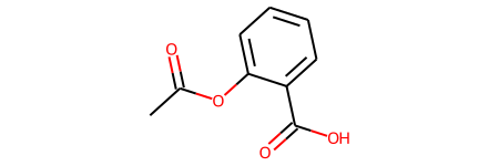
print(f"Name:\t{df.name[100]}\nSMILES:\t{df.smiles[100]}\nBBBP:\t{df.p_np[100]}")
molecule = molecule_from_smiles(df.iloc[100].smiles)
print("Molecule:")
molecule
Name:   acetylsalicylate
SMILES: CC(=O)Oc1ccccc1C(O)=O
BBBP:   0
Molecule:
graph = graph_from_molecule(molecule)
print("Graph (including self-loops):")
print("\tatom features\t", graph[0].shape)
print("\tbond features\t", graph[1].shape)
print("\tpair indices\t", graph[2].shape)
Graph (including self-loops):
    atom features    (13, 29)
    bond features    (39, 7)
    pair indices     (39, 2)
创建 tf.data.Dataset
在本教程中,MPNN 实现将(每次迭代)以单个图作为输入。因此,给定一批(子)图(分子),我们需要将它们合并成一个图(我们将这个图称为全局图)。这个全局图是一个不连通的图,其中每个子图与其他子图完全分开。
def prepare_batch(x_batch, y_batch):
    """Merges (sub)graphs of batch into a single global (disconnected) graph
    """

    atom_features, bond_features, pair_indices = x_batch

    # Obtain number of atoms and bonds for each graph (molecule)
    num_atoms = atom_features.row_lengths()
    num_bonds = bond_features.row_lengths()

    # Obtain partition indices (molecule_indicator), which will be used to
    # gather (sub)graphs from global graph in model later on
    molecule_indices = tf.range(len(num_atoms))
    molecule_indicator = tf.repeat(molecule_indices, num_atoms)

    # Merge (sub)graphs into a global (disconnected) graph. Adding 'increment' to
    # 'pair_indices' (and merging ragged tensors) actualizes the global graph
    gather_indices = tf.repeat(molecule_indices[:-1], num_bonds[1:])
    increment = tf.cumsum(num_atoms[:-1])
    increment = tf.pad(tf.gather(increment, gather_indices), [(num_bonds[0], 0)])
    pair_indices = pair_indices.merge_dims(outer_axis=0, inner_axis=1).to_tensor()
    pair_indices = pair_indices + increment[:, tf.newaxis]
    atom_features = atom_features.merge_dims(outer_axis=0, inner_axis=1).to_tensor()
    bond_features = bond_features.merge_dims(outer_axis=0, inner_axis=1).to_tensor()

    return (atom_features, bond_features, pair_indices, molecule_indicator), y_batch


def MPNNDataset(X, y, batch_size=32, shuffle=False):
    dataset = tf.data.Dataset.from_tensor_slices((X, (y)))
    if shuffle:
        dataset = dataset.shuffle(1024)
    return dataset.batch(batch_size).map(prepare_batch, -1).prefetch(-1)
模型
MPNN 模型可以有各种形状和形式。在本教程中,我们将实现一个基于原始论文 Neural Message Passing for Quantum Chemistry 和 DeepChem's MPNNModel 的 MPNN。本教程的 MPNN 由三个阶段组成:消息传递、读出和分类。
消息传递
消息传递步骤本身包括两个部分:
-
边网络,它根据它们之间的边特征 (
e_{vw_{i}}) 将消息从v的 1 跳邻居w_{i}传递到v,从而得到更新的节点(状态)v'。w_{i}表示v的第i个邻居。 -
门控循环单元(GRU),它接收最新的节点状态作为输入,并根据先前的节点状态更新它。换句话说,最新的节点状态充当 GRU 的输入,而先前的节点状态则包含在 GRU 的内存状态中。这使得信息可以从一个节点状态(例如,
v)传播到另一个节点状态(例如,v'')。
重要的是,步骤(1)和(2)会重复 k 步,并且在每一步 1...k,从 v 聚合信息的半径(或跳数)会增加 1。
class EdgeNetwork(layers.Layer):
    def build(self, input_shape):
        self.atom_dim = input_shape[0][-1]
        self.bond_dim = input_shape[1][-1]
        self.kernel = self.add_weight(
            shape=(self.bond_dim, self.atom_dim * self.atom_dim),
            initializer="glorot_uniform",
            name="kernel",
        )
        self.bias = self.add_weight(
            shape=(self.atom_dim * self.atom_dim), initializer="zeros", name="bias",
        )
        self.built = True

    def call(self, inputs):
        atom_features, bond_features, pair_indices = inputs

        # Apply linear transformation to bond features
        bond_features = tf.matmul(bond_features, self.kernel) + self.bias

        # Reshape for neighborhood aggregation later
        bond_features = tf.reshape(bond_features, (-1, self.atom_dim, self.atom_dim))

        # Obtain atom features of neighbors
        atom_features_neighbors = tf.gather(atom_features, pair_indices[:, 1])
        atom_features_neighbors = tf.expand_dims(atom_features_neighbors, axis=-1)

        # Apply neighborhood aggregation
        transformed_features = tf.matmul(bond_features, atom_features_neighbors)
        transformed_features = tf.squeeze(transformed_features, axis=-1)
        aggregated_features = tf.math.unsorted_segment_sum(
            transformed_features,
            pair_indices[:, 0],
            num_segments=tf.shape(atom_features)[0],
        )
        return aggregated_features


class MessagePassing(layers.Layer):
    def __init__(self, units, steps=4, **kwargs):
        super().__init__(**kwargs)
        self.units = units
        self.steps = steps

    def build(self, input_shape):
        self.atom_dim = input_shape[0][-1]
        self.message_step = EdgeNetwork()
        self.pad_length = max(0, self.units - self.atom_dim)
        self.update_step = layers.GRUCell(self.atom_dim + self.pad_length)
        self.built = True

    def call(self, inputs):
        atom_features, bond_features, pair_indices = inputs

        # Pad atom features if number of desired units exceeds atom_features dim.
        # Alternatively, a dense layer could be used here.
        atom_features_updated = tf.pad(atom_features, [(0, 0), (0, self.pad_length)])

        # Perform a number of steps of message passing
        for i in range(self.steps):
            # Aggregate information from neighbors
            atom_features_aggregated = self.message_step(
                [atom_features_updated, bond_features, pair_indices]
            )

            # Update node state via a step of GRU
            atom_features_updated, _ = self.update_step(
                atom_features_aggregated, atom_features_updated
            )
        return atom_features_updated
读出
当消息传递过程结束时,将 k 步聚合的节点状态分区到子图中(对应于批次中的每个分子),然后将其缩减到图级嵌入。在 原始论文中,为此目的使用了 集对集层。然而,在本教程中,将使用 Transformer 编码器 + 平均池化。具体来说:
- 将 k 步聚合的节点状态分区到子图中(对应于批次中的每个分子);
- 然后将每个子图填充到与节点最多的子图匹配,然后进行
tf.stack(...); - (填充后的堆叠)张量,其中编码了子图(每个子图包含一组节点状态),会被屏蔽,以确保填充不会干扰训练;
- 最后,将张量传递给 Transformer,然后进行平均池化。
class PartitionPadding(layers.Layer):
    def __init__(self, batch_size, **kwargs):
        super().__init__(**kwargs)
        self.batch_size = batch_size

    def call(self, inputs):

        atom_features, molecule_indicator = inputs

        # Obtain subgraphs
        atom_features_partitioned = tf.dynamic_partition(
            atom_features, molecule_indicator, self.batch_size
        )

        # Pad and stack subgraphs
        num_atoms = [tf.shape(f)[0] for f in atom_features_partitioned]
        max_num_atoms = tf.reduce_max(num_atoms)
        atom_features_stacked = tf.stack(
            [
                tf.pad(f, [(0, max_num_atoms - n), (0, 0)])
                for f, n in zip(atom_features_partitioned, num_atoms)
            ],
            axis=0,
        )

        # Remove empty subgraphs (usually for last batch in dataset)
        gather_indices = tf.where(tf.reduce_sum(atom_features_stacked, (1, 2)) != 0)
        gather_indices = tf.squeeze(gather_indices, axis=-1)
        return tf.gather(atom_features_stacked, gather_indices, axis=0)


class TransformerEncoderReadout(layers.Layer):
    def __init__(
        self, num_heads=8, embed_dim=64, dense_dim=512, batch_size=32, **kwargs
    ):
        super().__init__(**kwargs)

        self.partition_padding = PartitionPadding(batch_size)
        self.attention = layers.MultiHeadAttention(num_heads, embed_dim)
        self.dense_proj = keras.Sequential(
            [layers.Dense(dense_dim, activation="relu"), layers.Dense(embed_dim),]
        )
        self.layernorm_1 = layers.LayerNormalization()
        self.layernorm_2 = layers.LayerNormalization()
        self.average_pooling = layers.GlobalAveragePooling1D()

    def call(self, inputs):
        x = self.partition_padding(inputs)
        padding_mask = tf.reduce_any(tf.not_equal(x, 0.0), axis=-1)
        padding_mask = padding_mask[:, tf.newaxis, tf.newaxis, :]
        attention_output = self.attention(x, x, attention_mask=padding_mask)
        proj_input = self.layernorm_1(x + attention_output)
        proj_output = self.layernorm_2(proj_input + self.dense_proj(proj_input))
        return self.average_pooling(proj_output)
消息传递神经网络 (MPNN)
现在是时候完成 MPNN 模型了。除了消息传递和读出,还将实现一个两层分类网络来预测 BBBP。
def MPNNModel(
atom_dim,
bond_dim,
batch_size=32,
message_units=64,
message_steps=4,
num_attention_heads=8,
dense_units=512,
):
atom_features = layers.Input((atom_dim), dtype="float32", name="atom_features")
bond_features = layers.Input((bond_dim), dtype="float32", name="bond_features")
pair_indices = layers.Input((2), dtype="int32", name="pair_indices")
molecule_indicator = layers.Input((), dtype="int32", name="molecule_indicator")
x = MessagePassing(message_units, message_steps)(
[atom_features, bond_features, pair_indices]
)
x = TransformerEncoderReadout(
num_attention_heads, message_units, dense_units, batch_size
)([x, molecule_indicator])
x = layers.Dense(dense_units, activation="relu")(x)
x = layers.Dense(1, activation="sigmoid")(x)
model = keras.Model(
inputs=[atom_features, bond_features, pair_indices, molecule_indicator],
outputs=[x],
)
return model
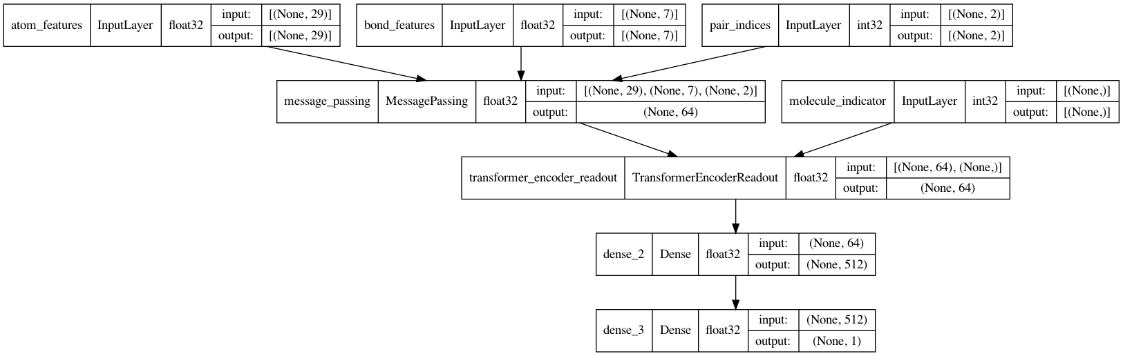
mpnn = MPNNModel(
atom_dim=x_train[0][0][0].shape[0], bond_dim=x_train[1][0][0].shape[0],
)
mpnn.compile(
loss=keras.losses.BinaryCrossentropy(),
optimizer=keras.optimizers.Adam(learning_rate=5e-4),
metrics=[keras.metrics.AUC(name="AUC")],
)
keras.utils.plot_model(mpnn, show_dtype=True, show_shapes=True)
训练
train_dataset = MPNNDataset(x_train, y_train)
valid_dataset = MPNNDataset(x_valid, y_valid)
test_dataset = MPNNDataset(x_test, y_test)
history = mpnn.fit(
train_dataset,
validation_data=valid_dataset,
epochs=40,
verbose=2,
class_weight={0: 2.0, 1: 0.5},
)
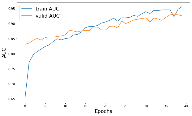
plt.figure(figsize=(10, 6))
plt.plot(history.history["AUC"], label="train AUC")
plt.plot(history.history["val_AUC"], label="valid AUC")
plt.xlabel("Epochs", fontsize=16)
plt.ylabel("AUC", fontsize=16)
plt.legend(fontsize=16)
Epoch 1/40
52/52 - 26s - loss: 0.5572 - AUC: 0.6527 - val_loss: 0.4660 - val_AUC: 0.8312 - 26s/epoch - 501ms/step
Epoch 2/40
52/52 - 22s - loss: 0.4817 - AUC: 0.7713 - val_loss: 0.6889 - val_AUC: 0.8351 - 22s/epoch - 416ms/step
Epoch 3/40
52/52 - 24s - loss: 0.4611 - AUC: 0.7960 - val_loss: 0.5863 - val_AUC: 0.8444 - 24s/epoch - 457ms/step
Epoch 4/40
52/52 - 19s - loss: 0.4493 - AUC: 0.8069 - val_loss: 0.5059 - val_AUC: 0.8509 - 19s/epoch - 372ms/step
Epoch 5/40
52/52 - 21s - loss: 0.4420 - AUC: 0.8155 - val_loss: 0.4965 - val_AUC: 0.8454 - 21s/epoch - 405ms/step
Epoch 6/40
52/52 - 22s - loss: 0.4344 - AUC: 0.8243 - val_loss: 0.5307 - val_AUC: 0.8540 - 22s/epoch - 419ms/step
Epoch 7/40
52/52 - 26s - loss: 0.4301 - AUC: 0.8293 - val_loss: 0.5131 - val_AUC: 0.8559 - 26s/epoch - 503ms/step
Epoch 8/40
52/52 - 31s - loss: 0.4163 - AUC: 0.8408 - val_loss: 0.5361 - val_AUC: 0.8552 - 31s/epoch - 599ms/step
Epoch 9/40
52/52 - 30s - loss: 0.4095 - AUC: 0.8499 - val_loss: 0.5371 - val_AUC: 0.8572 - 30s/epoch - 578ms/step
Epoch 10/40
52/52 - 23s - loss: 0.4107 - AUC: 0.8459 - val_loss: 0.5923 - val_AUC: 0.8589 - 23s/epoch - 444ms/step
Epoch 11/40
52/52 - 29s - loss: 0.4107 - AUC: 0.8505 - val_loss: 0.5070 - val_AUC: 0.8627 - 29s/epoch - 553ms/step
Epoch 12/40
52/52 - 25s - loss: 0.4005 - AUC: 0.8522 - val_loss: 0.5417 - val_AUC: 0.8781 - 25s/epoch - 471ms/step
Epoch 13/40
52/52 - 22s - loss: 0.3924 - AUC: 0.8623 - val_loss: 0.5915 - val_AUC: 0.8755 - 22s/epoch - 425ms/step
Epoch 14/40
52/52 - 19s - loss: 0.3872 - AUC: 0.8640 - val_loss: 0.5852 - val_AUC: 0.8724 - 19s/epoch - 365ms/step
Epoch 15/40
52/52 - 19s - loss: 0.3812 - AUC: 0.8720 - val_loss: 0.4949 - val_AUC: 0.8759 - 19s/epoch - 362ms/step
Epoch 16/40
52/52 - 27s - loss: 0.3604 - AUC: 0.8864 - val_loss: 0.5076 - val_AUC: 0.8773 - 27s/epoch - 521ms/step
Epoch 17/40
52/52 - 37s - loss: 0.3554 - AUC: 0.8907 - val_loss: 0.4556 - val_AUC: 0.8771 - 37s/epoch - 712ms/step
Epoch 18/40
52/52 - 23s - loss: 0.3554 - AUC: 0.8904 - val_loss: 0.4854 - val_AUC: 0.8887 - 23s/epoch - 452ms/step
Epoch 19/40
52/52 - 26s - loss: 0.3504 - AUC: 0.8942 - val_loss: 0.4622 - val_AUC: 0.8881 - 26s/epoch - 507ms/step
Epoch 20/40
52/52 - 20s - loss: 0.3378 - AUC: 0.9019 - val_loss: 0.5568 - val_AUC: 0.8792 - 20s/epoch - 390ms/step
Epoch 21/40
52/52 - 19s - loss: 0.3324 - AUC: 0.9055 - val_loss: 0.5623 - val_AUC: 0.8789 - 19s/epoch - 363ms/step
Epoch 22/40
52/52 - 19s - loss: 0.3248 - AUC: 0.9109 - val_loss: 0.5486 - val_AUC: 0.8909 - 19s/epoch - 357ms/step
Epoch 23/40
52/52 - 18s - loss: 0.3126 - AUC: 0.9179 - val_loss: 0.5684 - val_AUC: 0.8916 - 18s/epoch - 348ms/step
Epoch 24/40
52/52 - 18s - loss: 0.3296 - AUC: 0.9084 - val_loss: 0.5462 - val_AUC: 0.8858 - 18s/epoch - 352ms/step
Epoch 25/40
52/52 - 18s - loss: 0.3098 - AUC: 0.9193 - val_loss: 0.4212 - val_AUC: 0.9085 - 18s/epoch - 349ms/step
Epoch 26/40
52/52 - 18s - loss: 0.3095 - AUC: 0.9192 - val_loss: 0.4991 - val_AUC: 0.9002 - 18s/epoch - 348ms/step
Epoch 27/40
52/52 - 18s - loss: 0.3056 - AUC: 0.9211 - val_loss: 0.4739 - val_AUC: 0.9060 - 18s/epoch - 349ms/step
Epoch 28/40
52/52 - 18s - loss: 0.2942 - AUC: 0.9270 - val_loss: 0.4188 - val_AUC: 0.9121 - 18s/epoch - 344ms/step
Epoch 29/40
52/52 - 18s - loss: 0.3004 - AUC: 0.9241 - val_loss: 0.4056 - val_AUC: 0.9146 - 18s/epoch - 351ms/step
Epoch 30/40
52/52 - 18s - loss: 0.2810 - AUC: 0.9328 - val_loss: 0.3923 - val_AUC: 0.9172 - 18s/epoch - 355ms/step
Epoch 31/40
52/52 - 18s - loss: 0.2661 - AUC: 0.9398 - val_loss: 0.3609 - val_AUC: 0.9186 - 18s/epoch - 349ms/step
Epoch 32/40
52/52 - 19s - loss: 0.2797 - AUC: 0.9336 - val_loss: 0.3764 - val_AUC: 0.9055 - 19s/epoch - 357ms/step
Epoch 33/40
52/52 - 19s - loss: 0.2552 - AUC: 0.9441 - val_loss: 0.3941 - val_AUC: 0.9187 - 19s/epoch - 368ms/step
Epoch 34/40
52/52 - 23s - loss: 0.2601 - AUC: 0.9435 - val_loss: 0.4128 - val_AUC: 0.9154 - 23s/epoch - 443ms/step
Epoch 35/40
52/52 - 32s - loss: 0.2533 - AUC: 0.9455 - val_loss: 0.4191 - val_AUC: 0.9109 - 32s/epoch - 615ms/step
Epoch 36/40
52/52 - 23s - loss: 0.2530 - AUC: 0.9459 - val_loss: 0.4276 - val_AUC: 0.9213 - 23s/epoch - 435ms/step
Epoch 37/40
52/52 - 31s - loss: 0.2531 - AUC: 0.9456 - val_loss: 0.3950 - val_AUC: 0.9292 - 31s/epoch - 593ms/step
Epoch 38/40
52/52 - 22s - loss: 0.3039 - AUC: 0.9229 - val_loss: 0.3114 - val_AUC: 0.9315 - 22s/epoch - 428ms/step
Epoch 39/40
52/52 - 20s - loss: 0.2477 - AUC: 0.9479 - val_loss: 0.3584 - val_AUC: 0.9292 - 20s/epoch - 391ms/step
Epoch 40/40
52/52 - 22s - loss: 0.2276 - AUC: 0.9565 - val_loss: 0.3279 - val_AUC: 0.9258 - 22s/epoch - 416ms/step

<matplotlib.legend.Legend at 0x1603c63d0>
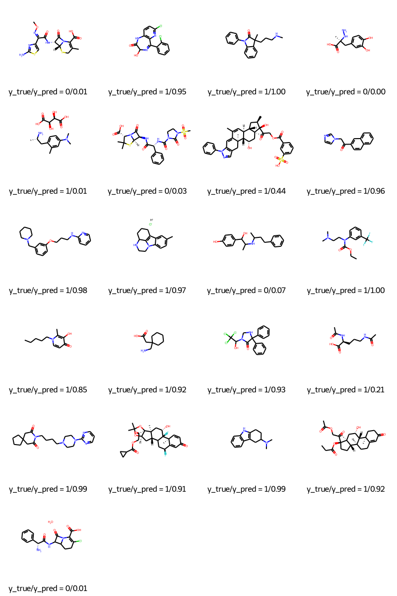
预测
molecules = [molecule_from_smiles(df.smiles.values[index]) for index in test_index]
y_true = [df.p_np.values[index] for index in test_index]
y_pred = tf.squeeze(mpnn.predict(test_dataset), axis=1)

legends = [f"y_true/y_pred = {y_true[i]}/{y_pred[i]:.2f}" for i in range(len(y_true))]
MolsToGridImage(molecules, molsPerRow=4, legends=legends)
结论
在本教程中,我们演示了一个消息传递神经网络 (MPNN),用于预测多种不同分子的血脑屏障通透性 (BBBP)。我们首先需要从 SMILES 构建图,然后构建一个能够处理这些图的 Keras 模型,最后训练模型进行预测。
HuggingFace 上提供的示例
| 训练好的模型 | 演示 |
|---|---|