► KerasRS / 示例 / 使用深度学习推荐模型进行排序

使用深度学习推荐模型进行排序

作者： Harshith Kulkarni
创建日期 2025/06/02
最后修改日期 2025/09/04
描述： 使用 KerasRS 对 DLRM 进行电影排序。

简介

本教程演示了如何使用深度学习推荐模型 (DLRM) 来有效地学习物品与用户偏好之间的关系，该模型使用点积交互机制。有关更多详细信息，请参阅 DLRM 论文。

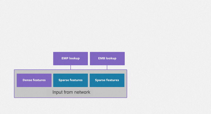
DLRM 旨在擅长捕获显式的、有界度的特征交互，并且在处理分类和连续（稀疏/密集）输入特征方面特别有效。该架构包含三个主要组件：用于处理各种特征的专用输入层（通常是分类特征的嵌入层）、用于显式建模特征交互的点积交互层，以及用于捕获隐式特征关系的（多层感知机）MLP。

点积交互层是 DLRM 的核心，它有效地计算不同特征嵌入之间的成对交互。这与深度和交叉网络 (DCN) 等模型不同，后者可以将特征向量内的元素视为独立单元，这可能会导致更高的维度空间和增加的计算成本。MLP 是标准的馈送网络。DLRM 由交互层和 MLP 组合而成。

下图展示了 DLRM 的架构

DLRM Architecture

现在我们对 DLRM 的架构和关键特征有了基础的了解，让我们深入研究代码。我们将使用真实世界的数据集训练一个 DLRM，以展示其学习有意义的特征交互的能力。让我们首先设置后端为 JAX 并组织我们的导入。

!pip install -q keras-rs

import os

os.environ["KERAS_BACKEND"] = "tensorflow"  # `"tensorflow"`/`"torch"`

import keras
import matplotlib.pyplot as plt
import numpy as np
import tensorflow as tf
import tensorflow_datasets as tfds
from mpl_toolkits.axes_grid1 import make_axes_locatable

import keras_rs

我们还可以定义将在整个示例中重复使用的变量。

MOVIELENS_CONFIG = {
    # features
    "continuous_features": [
        "raw_user_age",
        "hour_of_day_sin",
        "hour_of_day_cos",
        "hour_of_week_sin",
        "hour_of_week_cos",
    ],
    "categorical_int_features": [
        "user_gender",
    ],
    "categorical_str_features": [
        "user_zip_code",
        "user_occupation_text",
        "movie_id",
        "user_id",
    ],
    # model
    "embedding_dim": 8,
    "mlp_dim": 8,
    "deep_net_num_units": [192, 192, 192],
    # training
    "learning_rate": 1e-4,
    "num_epochs": 30,
    "batch_size": 8192,
}

在这里，我们定义一个辅助函数来可视化交叉层的权重，以便更好地理解其功能。此外，我们定义一个函数来编译、训练和评估给定的模型。

def plot_training_metrics(history):
    """Graphs all metrics tracked in the history object."""
    plt.figure(figsize=(12, 6))

    for metric_name, metric_values in history.history.items():
        plt.plot(metric_values, label=metric_name.replace("_", " ").title())

    plt.title("Metrics over Epochs")
    plt.xlabel("Epoch")
    plt.ylabel("Metric Value")
    plt.legend()
    plt.grid(True)


def visualize_layer(matrix, features, cmap=plt.cm.Blues):

    im = plt.matshow(
        matrix, cmap=cmap, extent=[-0.5, len(features) - 0.5, len(features) - 0.5, -0.5]
    )

    ax = plt.gca()
    divider = make_axes_locatable(plt.gca())
    cax = divider.append_axes("right", size="5%", pad=0.05)
    plt.colorbar(im, cax=cax)
    cax.tick_params(labelsize=10)

    # Set tick locations explicitly before setting labels
    ax.set_xticks(np.arange(len(features)))
    ax.set_yticks(np.arange(len(features)))

    ax.set_xticklabels(features, rotation=45, fontsize=5)
    ax.set_yticklabels(features, fontsize=5)

    plt.show()


def train_and_evaluate(
    learning_rate,
    epochs,
    train_data,
    test_data,
    model,
    plot_metrics=False,
):
    optimizer = keras.optimizers.AdamW(learning_rate=learning_rate, clipnorm=1.0)
    loss = keras.losses.MeanSquaredError()
    rmse = keras.metrics.RootMeanSquaredError()

    model.compile(
        optimizer=optimizer,
        loss=loss,
        metrics=[rmse],
    )

    history = model.fit(
        train_data,
        epochs=epochs,
        verbose=1,
    )
    if plot_metrics:
        plot_training_metrics(history)

    results = model.evaluate(test_data, return_dict=True, verbose=1)
    rmse_value = results["root_mean_squared_error"]

    return rmse_value, model.count_params()


def print_stats(rmse_list, num_params, model_name):
    # Report metrics.
    num_trials = len(rmse_list)
    avg_rmse = np.mean(rmse_list)
    std_rmse = np.std(rmse_list)

    if num_trials == 1:
        print(f"{model_name}: RMSE = {avg_rmse}; #params = {num_params}")
    else:
        print(f"{model_name}: RMSE = {avg_rmse} ± {std_rmse}; #params = {num_params}")

真实世界示例

让我们使用 MovieLens 100K 数据集。该数据集用于训练模型，根据用户相关特征和电影相关特征预测用户的电影评分。

准备数据集

这里的数据集处理步骤与基本排序教程中的步骤相似。让我们加载数据集，并只保留有用的列。

ratings_ds = tfds.load("movielens/100k-ratings", split="train")


def preprocess_features(x):
    """Extracts and cyclically encodes timestamp features."""
    features = {
        "movie_id": x["movie_id"],
        "user_id": x["user_id"],
        "user_gender": tf.cast(x["user_gender"], dtype=tf.int32),
        "user_zip_code": x["user_zip_code"],
        "user_occupation_text": x["user_occupation_text"],
        "raw_user_age": tf.cast(x["raw_user_age"], dtype=tf.float32),
    }
    label = tf.cast(x["user_rating"], dtype=tf.float32)

    # The timestamp is in seconds since the epoch.
    timestamp = tf.cast(x["timestamp"], dtype=tf.float32)

    # Constants for time periods
    SECONDS_IN_HOUR = 3600.0
    HOURS_IN_DAY = 24.0
    HOURS_IN_WEEK = 168.0

    # Calculate hour of day and encode it
    hour_of_day = (timestamp / SECONDS_IN_HOUR) % HOURS_IN_DAY
    features["hour_of_day_sin"] = tf.sin(2 * np.pi * hour_of_day / HOURS_IN_DAY)
    features["hour_of_day_cos"] = tf.cos(2 * np.pi * hour_of_day / HOURS_IN_DAY)

    # Calculate hour of week and encode it
    hour_of_week = (timestamp / SECONDS_IN_HOUR) % HOURS_IN_WEEK
    features["hour_of_week_sin"] = tf.sin(2 * np.pi * hour_of_week / HOURS_IN_WEEK)
    features["hour_of_week_cos"] = tf.cos(2 * np.pi * hour_of_week / HOURS_IN_WEEK)

    return features, label


# Apply the new preprocessing function
ratings_ds = ratings_ds.map(preprocess_features)

对于每个分类特征，让我们获取唯一值的列表，即词汇表，以便我们可以将其用于嵌入层。

vocabularies = {}
for feature_name in (
    MOVIELENS_CONFIG["categorical_int_features"]
    + MOVIELENS_CONFIG["categorical_str_features"]
):
    vocabulary = ratings_ds.batch(10_000).map(lambda x, y: x[feature_name])
    vocabularies[feature_name] = np.unique(np.concatenate(list(vocabulary)))

我们需要做的一件事是使用 keras.layers.StringLookup 和 keras.layers.IntegerLookup 将所有分类特征转换为索引，然后可以将这些索引馈送到嵌入层。

lookup_layers = {}
lookup_layers.update(
    {
        feature: keras.layers.IntegerLookup(vocabulary=vocabularies[feature])
        for feature in MOVIELENS_CONFIG["categorical_int_features"]
    }
)
lookup_layers.update(
    {
        feature: keras.layers.StringLookup(vocabulary=vocabularies[feature])
        for feature in MOVIELENS_CONFIG["categorical_str_features"]
    }
)

让我们标准化所有连续特征，以便我们可以将它们用于 MLP 层。

normalization_layers = {}
for feature_name in MOVIELENS_CONFIG["continuous_features"]:
    normalization_layers[feature_name] = keras.layers.Normalization(axis=-1)

training_data_for_adaptation = ratings_ds.take(80_000).map(lambda x, y: x)

for feature_name in MOVIELENS_CONFIG["continuous_features"]:
    feature_ds = training_data_for_adaptation.map(
        lambda x: tf.expand_dims(x[feature_name], axis=-1)
    )
    normalization_layers[feature_name].adapt(feature_ds)

ratings_ds = ratings_ds.map(
    lambda x, y: (
        {
            **{
                feature_name: lookup_layers[feature_name](x[feature_name])
                for feature_name in vocabularies
            },
            # Apply the adapted normalization layers to the continuous features.
            **{
                feature_name: tf.squeeze(
                    normalization_layers[feature_name](
                        tf.expand_dims(x[feature_name], axis=-1)
                    ),
                    axis=-1,
                )
                for feature_name in MOVIELENS_CONFIG["continuous_features"]
            },
        },
        y,
    )
)

让我们将数据拆分为训练集和测试集。我们还使用 cache() 和 prefetch() 以提高性能。

ratings_ds = ratings_ds.shuffle(100_000)

train_ds = (
    ratings_ds.take(80_000)
    .batch(MOVIELENS_CONFIG["batch_size"])
    .cache()
    .prefetch(tf.data.AUTOTUNE)
)
test_ds = (
    ratings_ds.skip(80_000)
    .batch(MOVIELENS_CONFIG["batch_size"])
    .take(20_000)
    .cache()
    .prefetch(tf.data.AUTOTUNE)
)

构建模型

模型将包含嵌入层，然后是 DotInteraction 和前馈层。

class DLRM(keras.Model):
    def __init__(
        self,
        dense_num_units_lst,
        embedding_dim=MOVIELENS_CONFIG["embedding_dim"],
        mlp_dim=MOVIELENS_CONFIG["mlp_dim"],
        **kwargs,
    ):
        super().__init__(**kwargs)

        self.embedding_layers = {}
        for feature_name in (
            MOVIELENS_CONFIG["categorical_int_features"]
            + MOVIELENS_CONFIG["categorical_str_features"]
        ):
            vocab_size = len(vocabularies[feature_name]) + 1  # +1 for OOV token
            self.embedding_layers[feature_name] = keras.layers.Embedding(
                input_dim=vocab_size,
                output_dim=embedding_dim,
            )

        self.bottom_mlp = keras.Sequential(
            [
                keras.layers.Dense(mlp_dim, activation="relu"),
                keras.layers.Dense(embedding_dim),  # Output must match embedding_dim
            ]
        )

        self.dot_layer = keras_rs.layers.DotInteraction()

        self.top_mlp = []
        for num_units in dense_num_units_lst:
            self.top_mlp.append(keras.layers.Dense(num_units, activation="relu"))

        self.output_layer = keras.layers.Dense(1)

        self.dense_num_units_lst = dense_num_units_lst
        self.embedding_dim = embedding_dim

    def call(self, inputs):
        embeddings = []
        for feature_name in (
            MOVIELENS_CONFIG["categorical_int_features"]
            + MOVIELENS_CONFIG["categorical_str_features"]
        ):
            embedding = self.embedding_layers[feature_name](inputs[feature_name])
            embeddings.append(embedding)

        # Process all continuous features together.
        continuous_inputs = []
        for feature_name in MOVIELENS_CONFIG["continuous_features"]:
            # Reshape each feature to (batch_size, 1)
            feature = keras.ops.reshape(
                keras.ops.cast(inputs[feature_name], dtype="float32"), (-1, 1)
            )
            continuous_inputs.append(feature)

        # Concatenate into a single tensor: (batch_size, num_continuous_features)
        concatenated_continuous = keras.ops.concatenate(continuous_inputs, axis=1)

        # Pass through the Bottom MLP to get one combined vector.
        processed_continuous = self.bottom_mlp(concatenated_continuous)

        # Combine with categorical embeddings. Note: we add a list containing the
        # single tensor.
        combined_features = embeddings + [processed_continuous]

        # Pass the list of features to the DotInteraction layer.
        x = self.dot_layer(combined_features)

        for layer in self.top_mlp:
            x = layer(x)

        x = self.output_layer(x)

        return x


dot_network = DLRM(
    dense_num_units_lst=MOVIELENS_CONFIG["deep_net_num_units"],
    embedding_dim=MOVIELENS_CONFIG["embedding_dim"],
    mlp_dim=MOVIELENS_CONFIG["mlp_dim"],
)

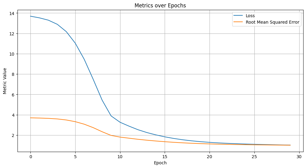
rmse, dot_network_num_params = train_and_evaluate(
    learning_rate=MOVIELENS_CONFIG["learning_rate"],
    epochs=MOVIELENS_CONFIG["num_epochs"],
    train_data=train_ds,
    test_data=test_ds,
    model=dot_network,
    plot_metrics=True,
)
print_stats(
    rmse_list=[rmse],
    num_params=dot_network_num_params,
    model_name="Dot Network",
)

png

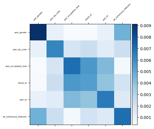
可视化特征交互

DotInteraction 层本身没有像 Dense 层那样的常规“权重”矩阵。相反，它的功能是计算你的特征的嵌入向量之间的点积。

为了可视化这些交互的强度，我们可以计算一个矩阵，该矩阵表示所有特征嵌入之间的成对交互强度。一种常见的方法是计算每对特征的嵌入矩阵的点积，然后将结果聚合为单个值（例如，绝对值的平均值），该值表示整体交互强度。

def get_dot_interaction_matrix(model, categorical_features, continuous_features):
    # The new feature list for the plot labels
    all_feature_names = categorical_features + ["all_continuous_features"]
    num_features = len(all_feature_names)

    # Store all feature outputs in the correct order.
    all_feature_outputs = []

    # Get outputs for categorical features from embedding layers (unchanged).
    for feature_name in categorical_features:
        embedding = model.embedding_layers[feature_name](keras.ops.array([0]))
        all_feature_outputs.append(embedding)

    # Get a single output for ALL continuous features from the shared MLP.
    num_continuous_features = len(continuous_features)
    # Create a dummy input of zeros for the MLP
    dummy_continuous_input = keras.ops.zeros((1, num_continuous_features))
    processed_continuous = model.bottom_mlp(dummy_continuous_input)
    all_feature_outputs.append(processed_continuous)

    interaction_matrix = np.zeros((num_features, num_features))

    # Iterate through each pair to calculate interaction strength.
    for i in range(num_features):
        for j in range(num_features):
            interaction = keras.ops.dot(
                all_feature_outputs[i], keras.ops.transpose(all_feature_outputs[j])
            )
            interaction_strength = keras.ops.convert_to_numpy(np.abs(interaction))[0][0]
            interaction_matrix[i, j] = interaction_strength

    return interaction_matrix, all_feature_names


# Get the list of categorical feature names.
categorical_feature_names = (
    MOVIELENS_CONFIG["categorical_int_features"]
    + MOVIELENS_CONFIG["categorical_str_features"]
)

# Calculate the interaction matrix with the corrected function.
interaction_matrix, feature_names = get_dot_interaction_matrix(
    model=dot_network,
    categorical_features=categorical_feature_names,
    continuous_features=MOVIELENS_CONFIG["continuous_features"],
)

# Visualize the matrix as a heatmap.
print("\nVisualizing the feature interaction strengths:")
visualize_layer(interaction_matrix, feature_names)

png

使用深度学习推荐模型进行排序

简介

真实世界示例

准备数据集

构建模型

可视化特征交互