使用迁移学习完成多项选择任务
作者: Md Awsafur Rahman
创建日期 2023/09/14
最后修改日期 2025/06/16
描述:使用预训练的 NLP 模型进行多项选择题任务。

简介
在此示例中,我们将演示如何通过微调预训练的 DebertaV3 模型来执行 **多项选择题** 任务。在此任务中,除了上下文外,还会提供几个候选答案,模型会进行训练以选择正确答案,这与问答任务不同。我们将使用 SWAG 数据集来演示此示例。
设置
import keras_hub
import keras
import tensorflow as tf  # For tf.data only.

import numpy as np
import pandas as pd

import matplotlib.pyplot as plt
数据集
在此示例中,我们将使用 **SWAG** 数据集进行多项选择题任务。
!wget "https://github.com/rowanz/swagaf/archive/refs/heads/master.zip" -O swag.zip
!unzip -q swag.zip
--2023-11-13 20:05:24--  https://github.com/rowanz/swagaf/archive/refs/heads/master.zip
Resolving github.com (github.com)... 192.30.255.113
Connecting to github.com (github.com)|192.30.255.113|:443... connected.
HTTP request sent, awaiting response... 302 Found
Location: https://codeload.github.com/rowanz/swagaf/zip/refs/heads/master [following]
--2023-11-13 20:05:25--  https://codeload.github.com/rowanz/swagaf/zip/refs/heads/master
Resolving codeload.github.com (codeload.github.com)... 20.29.134.24
Connecting to codeload.github.com (codeload.github.com)|20.29.134.24|:443... connected.
HTTP request sent, awaiting response... 200 OK
Length: unspecified [application/zip]
Saving to: ‘swag.zip’
swag.zip [ <=> ] 19.94M 4.25MB/s in 4.7s
2023-11-13 20:05:30 (4.25 MB/s) - ‘swag.zip’ saved [20905751]
!ls swagaf-master/data
README.md test.csv train.csv train_full.csv val.csv val_full.csv
配置
class CFG:
    preset = "deberta_v3_extra_small_en"  # Name of pretrained models
    sequence_length = 200  # Input sequence length
    seed = 42  # Random seed
    epochs = 5  # Training epochs
    batch_size = 8  # Batch size
    augment = True  # Augmentation (Shuffle Options)
可复现性
设置随机种子值,以在每次运行时产生类似的结果。
keras.utils.set_random_seed(CFG.seed)
元数据
- train.csv - 将用于训练。
sent1和sent2:这些字段显示了一个句子的开头,将两者结合起来,就得到了startphrase字段。ending_<i>:提出了句子可能结尾的几种可能选项,但只有一个是正确的。*label:标识正确的句子结尾。
- val.csv - 与
train.csv类似,但将用于验证。
# Train data
train_df = pd.read_csv(
    "swagaf-master/data/train.csv", index_col=0
)  # Read CSV file into a DataFrame
train_df = train_df.sample(frac=0.02)
print("# Train Data: {:,}".format(len(train_df)))

# Valid data
valid_df = pd.read_csv(
    "swagaf-master/data/val.csv", index_col=0
)  # Read CSV file into a DataFrame
valid_df = valid_df.sample(frac=0.02)
print("# Valid Data: {:,}".format(len(valid_df)))
# Train Data: 1,471
# Valid Data: 400
语境化选项
我们的方法是为模型提供问题和答案对,而不是为所有五个选项使用一个问题。在实践中,这意味着对于五个选项,我们将为模型提供相同的一组五个问题以及每个相应的答案选项(例如,(Q + A)、(Q + B) 等)。这种类比与在考试中多次回顾问题以促进对问题的深入理解的做法相似。
特别地,在 SWAG 数据集的上下文中,问题是句子的开头,而选项是句子可能结尾的选项。
# Define a function to create options based on the prompt and choices
def make_options(row):
    row["options"] = [
        f"{row.startphrase}\n{row.ending0}",  # Option 0
        f"{row.startphrase}\n{row.ending1}",  # Option 1
        f"{row.startphrase}\n{row.ending2}",  # Option 2
        f"{row.startphrase}\n{row.ending3}",
    ]  # Option 3
    return row
将 make_options 函数应用于数据帧的每一行
train_df = train_df.apply(make_options, axis=1)
valid_df = valid_df.apply(make_options, axis=1)
预处理
作用:预处理器接收输入字符串,并将其转换为包含预处理张量的字典(token_ids,padding_mask)。此过程从标记化开始,将输入字符串转换为标记 ID 序列。
重要性:最初,原始文本数据由于其高维度而变得复杂且难以建模。通过将文本转换为一组紧凑的标记,例如将 "The quick brown fox" 转换为 ["the", "qu", "##ick", "br", "##own", "fox"],我们简化了数据。许多模型依赖于特殊标记和其他张量来理解输入。这些标记有助于划分输入和识别填充等任务。通过填充使所有序列长度相同,可以提高计算效率,使后续步骤更顺畅。
探索以下页面,以访问 KerasHub 中可用的预处理和标记器层:- 预处理 - 标记器
preprocessor = keras_hub.models.DebertaV3Preprocessor.from_preset(
    preset=CFG.preset,  # Name of the model
    sequence_length=CFG.sequence_length,  # Max sequence length, will be padded if shorter
)
现在,让我们检查预处理层的输出形状是什么样的。层的输出形状可以表示为 $(num_choices, sequence_length)$。
outs = preprocessor(train_df.options.iloc[0])  # Process options for the first row

# Display the shape of each processed output
for k, v in outs.items():
    print(k, ":", v.shape)
CUDA backend failed to initialize: Found CUDA version 12010, but JAX was built against version 12020, which is newer. The copy of CUDA that is installed must be at least as new as the version against which JAX was built. (Set TF_CPP_MIN_LOG_LEVEL=0 and rerun for more info.)

token_ids : (4, 200)
padding_mask : (4, 200)
我们将使用 preprocessing_fn 函数通过 dataset.map(preprocessing_fn) 方法转换每个文本选项。
def preprocess_fn(text, label=None):
    text = preprocessor(text)  # Preprocess text
    return (
        (text, label) if label is not None else text
    )  # Return processed text and label if available
数据增强
在此笔记本中,我们将尝试一种有趣的增强技术,即 option_shuffle。由于我们一次向模型提供一个选项,因此我们可以对选项的顺序进行随机排序。例如,选项 [A, C, E, D, B] 将重新排列为 [D, B, A, E, C]。这种做法将有助于模型专注于选项本身的内容,而不是受到其位置的影响。
注意:尽管 option_shuffle 函数是用纯 TensorFlow 编写的,但它可以与任何后端(例如 JAX、PyTorch)一起使用,因为它仅在与 Keras 3 例程兼容的 tf.data.Dataset 流水线中使用。
def option_shuffle(options, labels, prob=0.50, seed=None):
    if tf.random.uniform([]) > prob:  # Shuffle probability check
        return options, labels
    # Shuffle indices of options and labels in the same order
    indices = tf.random.shuffle(tf.range(tf.shape(options)[0]), seed=seed)
    # Shuffle options and labels
    options = tf.gather(options, indices)
    labels = tf.gather(labels, indices)
    return options, labels
在以下函数中,我们将合并所有增强函数以应用于文本。这些增强将使用 dataset.map(augment_fn) 方法应用于数据。
def augment_fn(text, label=None):
    text, label = option_shuffle(text, label, prob=0.5)  # Shuffle the options
    return (text, label) if label is not None else text
数据加载器
以下代码使用 tf.data.Dataset 设置了一个强大的数据流流水线,用于数据处理。tf.data 的显著特点是它能够简化流水线构建并将组件表示为序列。
def build_dataset(
    texts,
    labels=None,
    batch_size=32,
    cache=False,
    augment=False,
    repeat=False,
    shuffle=1024,
):
    AUTO = tf.data.AUTOTUNE  # AUTOTUNE option
    slices = (
        (texts,)
        if labels is None
        else (texts, keras.utils.to_categorical(labels, num_classes=4))
    )  # Create slices
    ds = tf.data.Dataset.from_tensor_slices(slices)  # Create dataset from slices
    ds = ds.cache() if cache else ds  # Cache dataset if enabled
    if augment:  # Apply augmentation if enabled
        ds = ds.map(augment_fn, num_parallel_calls=AUTO)
    ds = ds.map(preprocess_fn, num_parallel_calls=AUTO)  # Map preprocessing function
    ds = ds.repeat() if repeat else ds  # Repeat dataset if enabled
    opt = tf.data.Options()  # Create dataset options
    if shuffle:
        ds = ds.shuffle(shuffle, seed=CFG.seed)  # Shuffle dataset if enabled
        opt.experimental_deterministic = False
    ds = ds.with_options(opt)  # Set dataset options
    ds = ds.batch(batch_size, drop_remainder=True)  # Batch dataset
    ds = ds.prefetch(AUTO)  # Prefetch next batch
    return ds  # Return the built dataset
现在让我们使用上述函数创建训练和验证数据加载器。
# Build train dataloader
train_texts = train_df.options.tolist()  # Extract training texts
train_labels = train_df.label.tolist()  # Extract training labels
train_ds = build_dataset(
    train_texts,
    train_labels,
    batch_size=CFG.batch_size,
    cache=True,
    shuffle=True,
    repeat=True,
    augment=CFG.augment,
)

# Build valid dataloader
valid_texts = valid_df.options.tolist()  # Extract validation texts
valid_labels = valid_df.label.tolist()  # Extract validation labels
valid_ds = build_dataset(
    valid_texts,
    valid_labels,
    batch_size=CFG.batch_size,
    cache=True,
    shuffle=False,
    repeat=False,
    augment=False,
)
学习率调度
实现学习率调度器对于迁移学习至关重要。学习率从 lr_start 开始,并使用 **余弦** 曲线逐渐减小到 lr_min。
重要性:结构良好的学习率调度器对于高效的模型训练至关重要,可确保最佳收敛并避免过冲或停滞等问题。
import math


def get_lr_callback(batch_size=8, mode="cos", epochs=10, plot=False):
    lr_start, lr_max, lr_min = 1.0e-6, 0.6e-6 * batch_size, 1e-6
    lr_ramp_ep, lr_sus_ep = 2, 0

    def lrfn(epoch):  # Learning rate update function
        if epoch < lr_ramp_ep:
            lr = (lr_max - lr_start) / lr_ramp_ep * epoch + lr_start
        elif epoch < lr_ramp_ep + lr_sus_ep:
            lr = lr_max
        else:
            decay_total_epochs, decay_epoch_index = (
                epochs - lr_ramp_ep - lr_sus_ep + 3,
                epoch - lr_ramp_ep - lr_sus_ep,
            )
            phase = math.pi * decay_epoch_index / decay_total_epochs
            lr = (lr_max - lr_min) * 0.5 * (1 + math.cos(phase)) + lr_min
        return lr

    if plot:  # Plot lr curve if plot is True
        plt.figure(figsize=(10, 5))
        plt.plot(
            np.arange(epochs),
            [lrfn(epoch) for epoch in np.arange(epochs)],
            marker="o",
        )
        plt.xlabel("epoch")
        plt.ylabel("lr")
        plt.title("LR Scheduler")
        plt.show()

    return keras.callbacks.LearningRateScheduler(
        lrfn, verbose=False
    )  # Create lr callback


_ = get_lr_callback(CFG.batch_size, plot=True)
![]()
回调
下面的函数将收集所有训练回调,例如 lr_scheduler、model_checkpoint。
def get_callbacks():
    callbacks = []
    lr_cb = get_lr_callback(CFG.batch_size)  # Get lr callback
    ckpt_cb = keras.callbacks.ModelCheckpoint(
        f"best.keras",
        monitor="val_accuracy",
        save_best_only=True,
        save_weights_only=False,
        mode="max",
    )  # Get Model checkpoint callback
    callbacks.extend([lr_cb, ckpt_cb])  # Add lr and checkpoint callbacks
    return callbacks  # Return the list of callbacks


callbacks = get_callbacks()
多项选择题模型
预训练模型
KerasHub 库提供了流行 NLP 模型架构的全面、现成的实现。它具有多种预训练模型,包括 Bert、Roberta、DebertaV3 等。在此笔记本中,我们将展示 DistillBert 的用法。但是,请随时在 KerasHub 文档 中探索所有可用的模型。另外,为了更深入地理解 KerasHub,请参阅信息丰富的 入门指南。
我们的方法包括使用 keras_hub.models.XXClassifier 来处理每个问题和选项对(例如 (Q+A)、(Q+B) 等),生成 logits。然后将这些 logits 组合并通过 softmax 函数得到最终输出。
多项选择题任务的分类器
在处理多项选择题时,我们不是将问题和所有选项一起提供给模型((Q + A + B + C ...)),而是将问题与一个选项一次性提供给模型。例如,(Q + A)、(Q + B) 等。一旦我们获得所有选项的预测分数(logits),我们就会使用 Softmax 函数将它们组合起来,得到最终结果。如果我们一次性将所有选项都提供给模型,文本的长度会增加,使模型难以处理。下图说明了这一点。
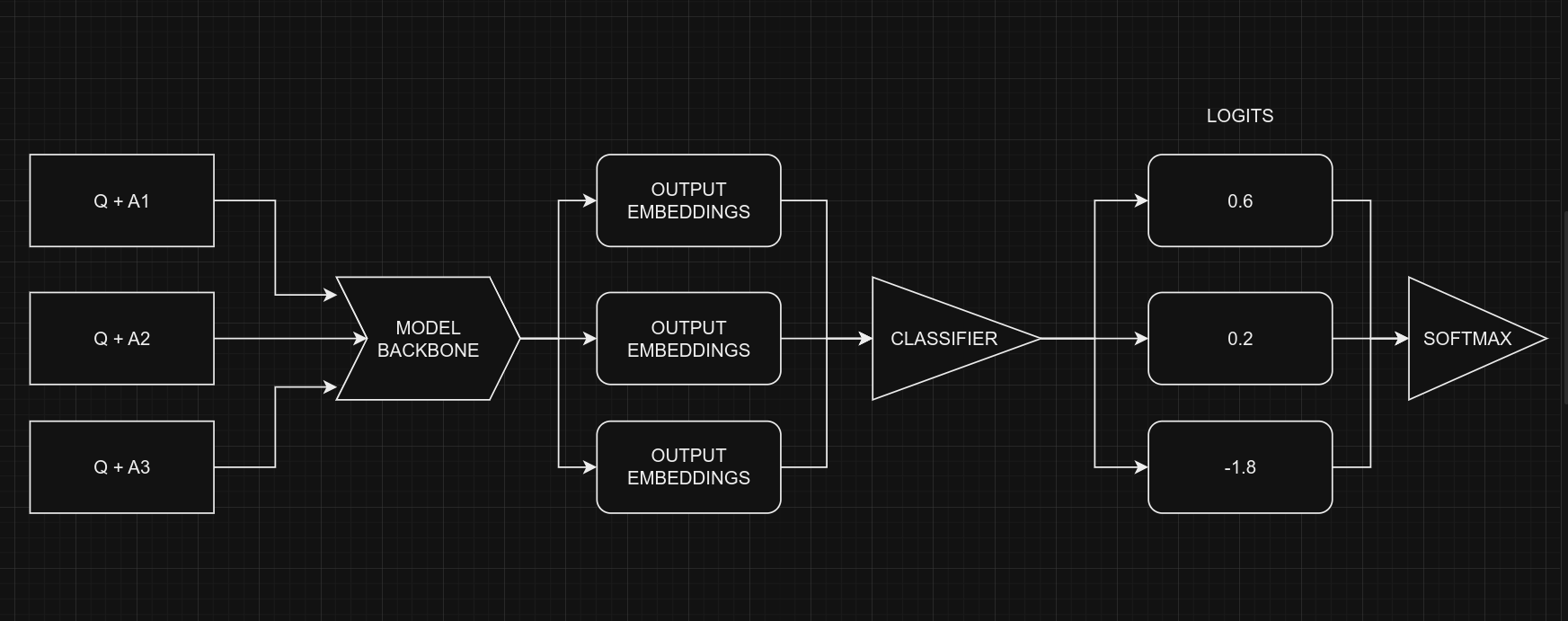
从编码的角度来看,请记住,我们对所有五个选项使用相同的模型,具有共享的权重。尽管图中显示了五个独立的模型,但它们实际上是一个具有共享权重的模型。另一点需要考虑的是 Classifier 和 MultipleChoice 的输入形状。
- 多项选择题的输入形状:$(batch_size, num_choices, seq_length)$
- 分类器的输入形状:$(batch_size, seq_length)$
当然,很明显我们不能直接将多项选择题的数据提供给模型,因为输入形状不匹配。为了处理这个问题,我们将使用 **切片**。这意味着我们将分离每个选项的特征,例如 $feature_{(Q + A)}$ 和 $feature_{(Q + B)}$,然后逐个提供给 NLP 分类器。在我们获得所有选项的预测分数 $logits_{(Q + A)}$ 和 $logits_{(Q + B)}$ 之后,我们将使用 Softmax 函数,例如 $\operatorname{Softmax}([logits_{(Q + A)}, logits_{(Q + B)}])$,将它们组合起来。这个最后一步有助于我们做出最终的决定或选择。
请注意,在分类器中,我们将
num_classes设置为1而不是5。这是因为分类器为每个选项产生一个单独的输出。当处理五个选项时,这些单独的输出会组合在一起,然后通过 softmax 函数进行处理以生成最终结果,其维度为5。
# Selects one option from five
class SelectOption(keras.layers.Layer):
    def __init__(self, index, **kwargs):
        super().__init__(**kwargs)
        self.index = index

    def call(self, inputs):
        # Selects a specific slice from the inputs tensor
        return inputs[:, self.index, :]

    def get_config(self):
        # For serialize the model
        base_config = super().get_config()
        config = {
            "index": self.index,
        }
        return {**base_config, **config}


def build_model():
    # Define input layers
    inputs = {
        "token_ids": keras.Input(shape=(4, None), dtype="int32", name="token_ids"),
        "padding_mask": keras.Input(
            shape=(4, None), dtype="int32", name="padding_mask"
        ),
    }
    # Create a DebertaV3Classifier model
    classifier = keras_hub.models.DebertaV3Classifier.from_preset(
        CFG.preset,
        preprocessor=None,
        num_classes=1,  # one output per one option, for five options total 5 outputs
    )
    logits = []
    # Loop through each option (Q+A), (Q+B) etc and compute associated logits
    for option_idx in range(4):
        option = {
            k: SelectOption(option_idx, name=f"{k}_{option_idx}")(v)
            for k, v in inputs.items()
        }
        logit = classifier(option)
        logits.append(logit)

    # Compute final output
    logits = keras.layers.Concatenate(axis=-1)(logits)
    outputs = keras.layers.Softmax(axis=-1)(logits)
    model = keras.Model(inputs, outputs)

    # Compile the model with optimizer, loss, and metrics
    model.compile(
        optimizer=keras.optimizers.AdamW(5e-6),
        loss=keras.losses.CategoricalCrossentropy(label_smoothing=0.02),
        metrics=[
            keras.metrics.CategoricalAccuracy(name="accuracy"),
        ],
        jit_compile=True,
    )
    return model


# Build the Build
model = build_model()
让我们检查模型摘要,以便更好地了解模型。
model.summary()
Model: "functional_1"
┏━━━━━━━━━━━━━━━━━━━━━┳━━━━━━━━━━━━━━━━━━━┳━━━━━━━━━┳━━━━━━━━━━━━━━━━━━━━━━┓
┃ Layer (type)        ┃ Output Shape      ┃ Param # ┃ Connected to         ┃
┡━━━━━━━━━━━━━━━━━━━━━╇━━━━━━━━━━━━━━━━━━━╇━━━━━━━━━╇━━━━━━━━━━━━━━━━━━━━━━┩
│ padding_mask        │ (None, 4, None)   │       0 │ -                    │
│ (InputLayer)        │                   │         │                      │
├─────────────────────┼───────────────────┼─────────┼──────────────────────┤
│ token_ids           │ (None, 4, None)   │       0 │ -                    │
│ (InputLayer)        │                   │         │                      │
├─────────────────────┼───────────────────┼─────────┼──────────────────────┤
│ padding_mask_0      │ (None, None)      │       0 │ padding_mask[0][0]   │
│ (SelectOption)      │                   │         │                      │
├─────────────────────┼───────────────────┼─────────┼──────────────────────┤
│ token_ids_0         │ (None, None)      │       0 │ token_ids[0][0]      │
│ (SelectOption)      │                   │         │                      │
├─────────────────────┼───────────────────┼─────────┼──────────────────────┤
│ padding_mask_1      │ (None, None)      │       0 │ padding_mask[0][0]   │
│ (SelectOption)      │                   │         │                      │
├─────────────────────┼───────────────────┼─────────┼──────────────────────┤
│ token_ids_1         │ (None, None)      │       0 │ token_ids[0][0]      │
│ (SelectOption)      │                   │         │                      │
├─────────────────────┼───────────────────┼─────────┼──────────────────────┤
│ padding_mask_2      │ (None, None)      │       0 │ padding_mask[0][0]   │
│ (SelectOption)      │                   │         │                      │
├─────────────────────┼───────────────────┼─────────┼──────────────────────┤
│ token_ids_2         │ (None, None)      │       0 │ token_ids[0][0]      │
│ (SelectOption)      │                   │         │                      │
├─────────────────────┼───────────────────┼─────────┼──────────────────────┤
│ padding_mask_3      │ (None, None)      │       0 │ padding_mask[0][0]   │
│ (SelectOption)      │                   │         │                      │
├─────────────────────┼───────────────────┼─────────┼──────────────────────┤
│ token_ids_3         │ (None, None)      │       0 │ token_ids[0][0]      │
│ (SelectOption)      │                   │         │                      │
├─────────────────────┼───────────────────┼─────────┼──────────────────────┤
│ deberta_v3_classif… │ (None, 1)         │ 70,830… │ padding_mask_0[0][0… │
│ (DebertaV3Classifi… │                   │         │ token_ids_0[0][0],   │
│                     │                   │         │ padding_mask_1[0][0… │
│                     │                   │         │ token_ids_1[0][0],   │
│                     │                   │         │ padding_mask_2[0][0… │
│                     │                   │         │ token_ids_2[0][0],   │
│                     │                   │         │ padding_mask_3[0][0… │
│                     │                   │         │ token_ids_3[0][0]    │
├─────────────────────┼───────────────────┼─────────┼──────────────────────┤
│ concatenate         │ (None, 4)         │       0 │ deberta_v3_classifi… │
│ (Concatenate)       │                   │         │ deberta_v3_classifi… │
│                     │                   │         │ deberta_v3_classifi… │
│                     │                   │         │ deberta_v3_classifi… │
├─────────────────────┼───────────────────┼─────────┼──────────────────────┤
│ softmax (Softmax)   │ (None, 4)         │       0 │ concatenate[0][0]    │
└─────────────────────┴───────────────────┴─────────┴──────────────────────┘
Total params: 70,830,337 (270.20 MB)
Trainable params: 70,830,337 (270.20 MB)
Non-trainable params: 0 (0.00 B)
最后,让我们直观地检查模型结构,以确保一切正常。
keras.utils.plot_model(model, show_shapes=True)
![]()
训练
# Start training the model
history = model.fit(
    train_ds,
    epochs=CFG.epochs,
    validation_data=valid_ds,
    callbacks=callbacks,
    steps_per_epoch=int(len(train_df) / CFG.batch_size),
    verbose=1,
)
Epoch 1/5
 183/183 ━━━━━━━━━━━━━━━━━━━━ 5087s 25s/step - accuracy: 0.2563 - loss: 1.3884 - val_accuracy: 0.5150 - val_loss: 1.3742 - learning_rate: 1.0000e-06
Epoch 2/5
 183/183 ━━━━━━━━━━━━━━━━━━━━ 4529s 25s/step - accuracy: 0.3825 - loss: 1.3364 - val_accuracy: 0.7125 - val_loss: 0.9071 - learning_rate: 2.9000e-06
Epoch 3/5
 183/183 ━━━━━━━━━━━━━━━━━━━━ 4524s 25s/step - accuracy: 0.6144 - loss: 1.0118 - val_accuracy: 0.7425 - val_loss: 0.8017 - learning_rate: 4.8000e-06
Epoch 4/5
 183/183 ━━━━━━━━━━━━━━━━━━━━ 4522s 25s/step - accuracy: 0.6744 - loss: 0.8460 - val_accuracy: 0.7625 - val_loss: 0.7323 - learning_rate: 4.7230e-06
Epoch 5/5
 183/183 ━━━━━━━━━━━━━━━━━━━━ 4517s 25s/step - accuracy: 0.7200 - loss: 0.7458 - val_accuracy: 0.7750 - val_loss: 0.7022 - learning_rate: 4.4984e-06
推理
# Make predictions using the trained model on last validation data
predictions = model.predict(
    valid_ds,
    batch_size=CFG.batch_size,  # max batch size = valid size
    verbose=1,
)

# Format predictions and true answers
pred_answers = np.arange(4)[np.argsort(-predictions)][:, 0]
true_answers = valid_df.label.values

# Check 5 Predictions
print("# Predictions\n")
for i in range(0, 50, 10):
    row = valid_df.iloc[i]
    question = row.startphrase
    pred_answer = f"ending{pred_answers[i]}"
    true_answer = f"ending{true_answers[i]}"
    print(f"❓ Sentence {i+1}:\n{question}\n")
    print(f"✅ True Ending: {true_answer}\n   >> {row[true_answer]}\n")
    print(f"🤖 Predicted Ending: {pred_answer}\n   >> {row[pred_answer]}\n")
    print("-" * 90, "\n")
 50/50 ━━━━━━━━━━━━━━━━━━━━ 274s 5s/step
# Predictions
❓ Sentence 1:
The man shows the teens how to move the oars. The teens
✅ True Ending: ending3
   >> follow the instructions of the man and row the oars.
🤖 Predicted Ending: ending3
   >> follow the instructions of the man and row the oars.
------------------------------------------------------------------------------------------
❓ Sentence 11:
A lake reflects the mountains and the sky. Someone
✅ True Ending: ending2
   >> runs along a desert highway.
🤖 Predicted Ending: ending1
   >> remains by the door.
------------------------------------------------------------------------------------------
❓ Sentence 21:
On screen, she smiles as someone holds up a present. He watches somberly as on screen, his mother
✅ True Ending: ending1
   >> picks him up and plays with him in the garden.
🤖 Predicted Ending: ending0
   >> comes out of her apartment, glowers at her laptop.
------------------------------------------------------------------------------------------
❓ Sentence 31:
A woman in a black shirt is sitting on a bench. A man
✅ True Ending: ending2
   >> sits behind a desk.
🤖 Predicted Ending: ending0
   >> is dancing on a stage.
------------------------------------------------------------------------------------------
❓ Sentence 41:
People are standing on sand wearing red shirts. They
✅ True Ending: ending3
   >> are playing a game of soccer in the sand.
🤖 Predicted Ending: ending3
   >> are playing a game of soccer in the sand.
------------------------------------------------------------------------------------------
参考
- 使用 HF 进行多项选择题
- Keras NLP
- BirdCLEF23:预训练是您所需要的一切 [训练] [训练]](https://www.kaggle.com/code/awsaf49/birdclef23-pretraining-is-all-you-need-train)
- 三重分层 KFold 与 TFRecords