内存高效的推荐系统嵌入
作者: Khalid Salama
创建日期 2021/02/15
最后修改日期 2023/11/15
描述: 使用组合式和混合维度嵌入来构建内存高效的推荐模型。

简介
本示例演示了两种通过减小嵌入表的大小来构建内存高效推荐模型的技巧,而不会牺牲模型效果。
- Hao-Jun Michael Shi 等人提出的商余数技巧,它减少了需要存储的嵌入向量的数量,但为每个项目生成了唯一的嵌入向量,而无需显式定义。
- Antonio Ginart 等人提出的混合维度嵌入,它存储了混合维度的嵌入向量,其中不太受欢迎的项目具有较低维度的嵌入。
我们使用了Movielens 数据集的 1M 版本。该数据集包含约 100 万条来自 6,000 名用户对 4,000 部电影的评分。
设置
import os

os.environ["KERAS_BACKEND"] = "tensorflow"

from zipfile import ZipFile
from urllib.request import urlretrieve
import numpy as np
import pandas as pd
import tensorflow as tf
import keras
from keras import layers
from keras.layers import StringLookup
import matplotlib.pyplot as plt
准备数据
下载和处理数据
urlretrieve("http://files.grouplens.org/datasets/movielens/ml-1m.zip", "movielens.zip")
ZipFile("movielens.zip", "r").extractall()

ratings_data = pd.read_csv(
    "ml-1m/ratings.dat",
    sep="::",
    names=["user_id", "movie_id", "rating", "unix_timestamp"],
)

ratings_data["movie_id"] = ratings_data["movie_id"].apply(lambda x: f"movie_{x}")
ratings_data["user_id"] = ratings_data["user_id"].apply(lambda x: f"user_{x}")
ratings_data["rating"] = ratings_data["rating"].apply(lambda x: float(x))
del ratings_data["unix_timestamp"]

print(f"Number of users: {len(ratings_data.user_id.unique())}")
print(f"Number of movies: {len(ratings_data.movie_id.unique())}")
print(f"Number of ratings: {len(ratings_data.index)}")
/var/folders/8n/8w8cqnvj01xd4ghznl11nyn000_93_/T/ipykernel_33554/2288473197.py:4: ParserWarning: Falling back to the 'python' engine because the 'c' engine does not support regex separators (separators > 1 char and different from '\s+' are interpreted as regex); you can avoid this warning by specifying engine='python'.
  ratings_data = pd.read_csv(

Number of users: 6040
Number of movies: 3706
Number of ratings: 1000209
创建训练和评估数据分割
random_selection = np.random.rand(len(ratings_data.index)) <= 0.85
train_data = ratings_data[random_selection]
eval_data = ratings_data[~random_selection]

train_data.to_csv("train_data.csv", index=False, sep="|", header=False)
eval_data.to_csv("eval_data.csv", index=False, sep="|", header=False)
print(f"Train data split: {len(train_data.index)}")
print(f"Eval data split: {len(eval_data.index)}")
print("Train and eval data files are saved.")
Train data split: 850573
Eval data split: 149636
Train and eval data files are saved.
定义数据集元数据和超参数
csv_header = list(ratings_data.columns)
user_vocabulary = list(ratings_data.user_id.unique())
movie_vocabulary = list(ratings_data.movie_id.unique())
target_feature_name = "rating"
learning_rate = 0.001
batch_size = 128
num_epochs = 3
base_embedding_dim = 64
训练和评估模型
def get_dataset_from_csv(csv_file_path, batch_size=128, shuffle=True):
    return tf.data.experimental.make_csv_dataset(
        csv_file_path,
        batch_size=batch_size,
        column_names=csv_header,
        label_name=target_feature_name,
        num_epochs=1,
        header=False,
        field_delim="|",
        shuffle=shuffle,
    )


def run_experiment(model):
    # Compile the model.
    model.compile(
        optimizer=keras.optimizers.Adam(learning_rate),
        loss=keras.losses.MeanSquaredError(),
        metrics=[keras.metrics.MeanAbsoluteError(name="mae")],
    )
    # Read the training data.
    train_dataset = get_dataset_from_csv("train_data.csv", batch_size)
    # Read the test data.
    eval_dataset = get_dataset_from_csv("eval_data.csv", batch_size, shuffle=False)
    # Fit the model with the training data.
    history = model.fit(
        train_dataset,
        epochs=num_epochs,
        validation_data=eval_dataset,
    )
    return history
实验 1:基线协同过滤模型
实现嵌入编码器
def embedding_encoder(vocabulary, embedding_dim, num_oov_indices=0, name=None):
    return keras.Sequential(
        [
            StringLookup(
                vocabulary=vocabulary, mask_token=None, num_oov_indices=num_oov_indices
            ),
            layers.Embedding(
                input_dim=len(vocabulary) + num_oov_indices, output_dim=embedding_dim
            ),
        ],
        name=f"{name}_embedding" if name else None,
    )
实现基线模型
def create_baseline_model():
    # Receive the user as an input.
    user_input = layers.Input(name="user_id", shape=(), dtype=tf.string)
    # Get user embedding.
    user_embedding = embedding_encoder(
        vocabulary=user_vocabulary, embedding_dim=base_embedding_dim, name="user"
    )(user_input)

    # Receive the movie as an input.
    movie_input = layers.Input(name="movie_id", shape=(), dtype=tf.string)
    # Get embedding.
    movie_embedding = embedding_encoder(
        vocabulary=movie_vocabulary, embedding_dim=base_embedding_dim, name="movie"
    )(movie_input)

    # Compute dot product similarity between user and movie embeddings.
    logits = layers.Dot(axes=1, name="dot_similarity")(
        [user_embedding, movie_embedding]
    )
    # Convert to rating scale.
    prediction = keras.activations.sigmoid(logits) * 5
    # Create the model.
    model = keras.Model(
        inputs=[user_input, movie_input], outputs=prediction, name="baseline_model"
    )
    return model


baseline_model = create_baseline_model()
baseline_model.summary()
/Users/fchollet/Library/Python/3.10/lib/python/site-packages/numpy/core/numeric.py:2468: FutureWarning: elementwise comparison failed; returning scalar instead, but in the future will perform elementwise comparison
  return bool(asarray(a1 == a2).all())
Model: "baseline_model"
┏━━━━━━━━━━━━━━━━━━━━━┳━━━━━━━━━━━━━━━━━━━┳━━━━━━━━━┳━━━━━━━━━━━━━━━━━━━━━━┓
┃ Layer (type)        ┃ Output Shape      ┃ Param # ┃ Connected to         ┃
┡━━━━━━━━━━━━━━━━━━━━━╇━━━━━━━━━━━━━━━━━━━╇━━━━━━━━━╇━━━━━━━━━━━━━━━━━━━━━━┩
│ user_id             │ (None)            │       0 │ -                    │
│ (InputLayer)        │                   │         │                      │
├─────────────────────┼───────────────────┼─────────┼──────────────────────┤
│ movie_id            │ (None)            │       0 │ -                    │
│ (InputLayer)        │                   │         │                      │
├─────────────────────┼───────────────────┼─────────┼──────────────────────┤
│ user_embedding      │ (None, 64)        │ 386,560 │ user_id[0][0]        │
│ (Sequential)        │                   │         │                      │
├─────────────────────┼───────────────────┼─────────┼──────────────────────┤
│ movie_embedding     │ (None, 64)        │ 237,184 │ movie_id[0][0]       │
│ (Sequential)        │                   │         │                      │
├─────────────────────┼───────────────────┼─────────┼──────────────────────┤
│ dot_similarity      │ (None, 1)         │       0 │ user_embedding[0][0… │
│ (Dot)               │                   │         │ movie_embedding[0][… │
├─────────────────────┼───────────────────┼─────────┼──────────────────────┤
│ sigmoid (Sigmoid)   │ (None, 1)         │       0 │ dot_similarity[0][0] │
├─────────────────────┼───────────────────┼─────────┼──────────────────────┤
│ multiply (Multiply) │ (None, 1)         │       0 │ sigmoid[0][0]        │
└─────────────────────┴───────────────────┴─────────┴──────────────────────┘
Total params: 623,744 (2.38 MB)
Trainable params: 623,744 (2.38 MB)
Non-trainable params: 0 (0.00 B)
请注意,可训练参数的数量为 623,744。
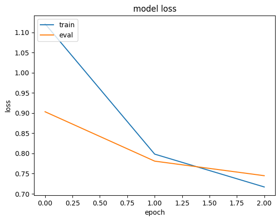
history = run_experiment(baseline_model)

plt.plot(history.history["loss"])
plt.plot(history.history["val_loss"])
plt.title("model loss")
plt.ylabel("loss")
plt.xlabel("epoch")
plt.legend(["train", "eval"], loc="upper left")
plt.show()
Epoch 1/3
   6629/Unknown  17s 3ms/step - loss: 1.4095 - mae: 0.9668

/Library/Frameworks/Python.framework/Versions/3.10/lib/python3.10/contextlib.py:153: UserWarning: Your input ran out of data; interrupting training. Make sure that your dataset or generator can generate at least `steps_per_epoch * epochs` batches. You may need to use the `.repeat()` function when building your dataset.
  self.gen.throw(typ, value, traceback)

 6646/6646 ━━━━━━━━━━━━━━━━━━━━ 18s 3ms/step - loss: 1.4087 - mae: 0.9665 - val_loss: 0.9032 - val_mae: 0.7438
Epoch 2/3
 6646/6646 ━━━━━━━━━━━━━━━━━━━━ 17s 3ms/step - loss: 0.8296 - mae: 0.7193 - val_loss: 0.7807 - val_mae: 0.6976
Epoch 3/3
 6646/6646 ━━━━━━━━━━━━━━━━━━━━ 17s 3ms/step - loss: 0.7305 - mae: 0.6744 - val_loss: 0.7446 - val_mae: 0.6808
实验 2:内存高效模型
将商余数嵌入实现为层
商余数技术的工作原理如下。对于一组词汇表和嵌入大小 `embedding_dim`,我们不创建 `vocabulary_size X embedding_dim` 的嵌入表,而是创建 *两个* `num_buckets X embedding_dim` 的嵌入表,其中 `num_buckets` 远小于 `vocabulary_size`。给定项目 `index` 的嵌入是通过以下步骤生成的:
- 计算 `quotient_index`,即 `index // num_buckets`。
- 计算 `remainder_index`,即 `index % num_buckets`。
- 使用 `quotient_index` 从第一个嵌入表中查找 `quotient_embedding`。
- 使用 `remainder_index` 从第二个嵌入表中查找 `remainder_embedding`。
- 返回 `quotient_embedding` * `remainder_embedding`。
这项技术不仅减少了需要存储和训练的嵌入向量的数量,而且为每个大小为 `embedding_dim` 的项目生成了*唯一*的嵌入向量。请注意,`q_embedding` 和 `r_embedding` 可以使用其他操作组合,例如 `Add` 和 `Concatenate`。
class QREmbedding(keras.layers.Layer):
    def __init__(self, vocabulary, embedding_dim, num_buckets, name=None):
        super().__init__(name=name)
        self.num_buckets = num_buckets

        self.index_lookup = StringLookup(
            vocabulary=vocabulary, mask_token=None, num_oov_indices=0
        )
        self.q_embeddings = layers.Embedding(
            num_buckets,
            embedding_dim,
        )
        self.r_embeddings = layers.Embedding(
            num_buckets,
            embedding_dim,
        )

    def call(self, inputs):
        # Get the item index.
        embedding_index = self.index_lookup(inputs)
        # Get the quotient index.
        quotient_index = tf.math.floordiv(embedding_index, self.num_buckets)
        # Get the reminder index.
        remainder_index = tf.math.floormod(embedding_index, self.num_buckets)
        # Lookup the quotient_embedding using the quotient_index.
        quotient_embedding = self.q_embeddings(quotient_index)
        # Lookup the remainder_embedding using the remainder_index.
        remainder_embedding = self.r_embeddings(remainder_index)
        # Use multiplication as a combiner operation
        return quotient_embedding * remainder_embedding
将混合维度嵌入实现为层
在混合维度嵌入技术中,我们为频繁查询的项目训练具有完整维度的嵌入向量,同时为不常查询的项目训练具有*降低维度*的嵌入向量,外加一个*投影权重矩阵*,将低维度嵌入转换为完整维度。
更具体地说,我们定义了相似频率的项目*块*。对于每个块,将创建一个 `block_vocab_size X block_embedding_dim` 的嵌入表和 `block_embedding_dim X full_embedding_dim` 的投影权重矩阵。请注意,如果 `block_embedding_dim` 等于 `full_embedding_dim`,则投影权重矩阵将成为*单位*矩阵。给定项目*索引*批次的嵌入是通过以下步骤生成的:
- 对于每个块,使用 `indices` 查找 `block_embedding_dim` 嵌入向量,并将其投影到 `full_embedding_dim`。
- 如果项目索引不属于某个块,则返回一个词汇表外嵌入。每个块将返回一个 `batch_size X full_embedding_dim` 的张量。
- 将掩码应用于从每个块返回的嵌入,以将词汇表外嵌入转换为零向量。也就是说,对于批次中的每个项目,从所有块嵌入中返回一个非零嵌入向量。
- 使用*求和*组合从块中检索的嵌入,以生成最终的 `batch_size X full_embedding_dim` 张量。
class MDEmbedding(keras.layers.Layer):
    def __init__(
        self, blocks_vocabulary, blocks_embedding_dims, base_embedding_dim, name=None
    ):
        super().__init__(name=name)
        self.num_blocks = len(blocks_vocabulary)

        # Create vocab to block lookup.
        keys = []
        values = []
        for block_idx, block_vocab in enumerate(blocks_vocabulary):
            keys.extend(block_vocab)
            values.extend([block_idx] * len(block_vocab))
        self.vocab_to_block = tf.lookup.StaticHashTable(
            tf.lookup.KeyValueTensorInitializer(keys, values), default_value=-1
        )

        self.block_embedding_encoders = []
        self.block_embedding_projectors = []

        # Create block embedding encoders and projectors.
        for idx in range(self.num_blocks):
            vocabulary = blocks_vocabulary[idx]
            embedding_dim = blocks_embedding_dims[idx]
            block_embedding_encoder = embedding_encoder(
                vocabulary, embedding_dim, num_oov_indices=1
            )
            self.block_embedding_encoders.append(block_embedding_encoder)
            if embedding_dim == base_embedding_dim:
                self.block_embedding_projectors.append(layers.Lambda(lambda x: x))
            else:
                self.block_embedding_projectors.append(
                    layers.Dense(units=base_embedding_dim)
                )

    def call(self, inputs):
        # Get block index for each input item.
        block_indicies = self.vocab_to_block.lookup(inputs)
        # Initialize output embeddings to zeros.
        embeddings = tf.zeros(shape=(tf.shape(inputs)[0], base_embedding_dim))
        # Generate embeddings from blocks.
        for idx in range(self.num_blocks):
            # Lookup embeddings from the current block.
            block_embeddings = self.block_embedding_encoders[idx](inputs)
            # Project embeddings to base_embedding_dim.
            block_embeddings = self.block_embedding_projectors[idx](block_embeddings)
            # Create a mask to filter out embeddings of items that do not belong to the current block.
            mask = tf.expand_dims(tf.cast(block_indicies == idx, tf.dtypes.float32), 1)
            # Set the embeddings for the items not belonging to the current block to zeros.
            block_embeddings = block_embeddings * mask
            # Add the block embeddings to the final embeddings.
            embeddings += block_embeddings

        return embeddings
实现内存高效模型
在此实验中,我们将使用**商余数**技术来减小用户嵌入的大小,并使用**混合维度**技术来减小电影嵌入的大小。
虽然在论文中,使用 alpha-power 规则来确定每个块嵌入的维度,但我们仅根据电影流行度的直方图可视化来设置块的数量和每个块的嵌入维度。
movie_frequencies = ratings_data["movie_id"].value_counts()
movie_frequencies.hist(bins=10)
<Axes: >
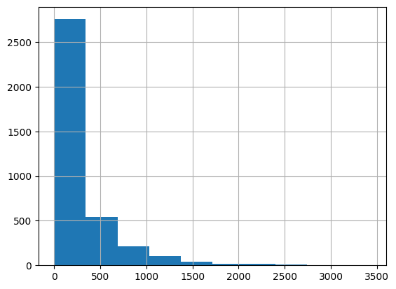
您可以看到,我们可以将电影分为三个块,并分别为它们分配 64、32 和 16 的嵌入维度。随意尝试不同的块数和维度。
sorted_movie_vocabulary = list(movie_frequencies.keys())

movie_blocks_vocabulary = [
    sorted_movie_vocabulary[:400],  # high popularity movies block
    sorted_movie_vocabulary[400:1700],  # normal popularity movies block
    sorted_movie_vocabulary[1700:],  # low popularity movies block
]

movie_blocks_embedding_dims = [64, 32, 16]

user_embedding_num_buckets = len(user_vocabulary) // 50


def create_memory_efficient_model():
    # Take the user as an input.
    user_input = layers.Input(name="user_id", shape=(), dtype="string")
    # Get user embedding.
    user_embedding = QREmbedding(
        vocabulary=user_vocabulary,
        embedding_dim=base_embedding_dim,
        num_buckets=user_embedding_num_buckets,
        name="user_embedding",
    )(user_input)

    # Take the movie as an input.
    movie_input = layers.Input(name="movie_id", shape=(), dtype="string")
    # Get embedding.
    movie_embedding = MDEmbedding(
        blocks_vocabulary=movie_blocks_vocabulary,
        blocks_embedding_dims=movie_blocks_embedding_dims,
        base_embedding_dim=base_embedding_dim,
        name="movie_embedding",
    )(movie_input)

    # Compute dot product similarity between user and movie embeddings.
    logits = layers.Dot(axes=1, name="dot_similarity")(
        [user_embedding, movie_embedding]
    )
    # Convert to rating scale.
    prediction = keras.activations.sigmoid(logits) * 5
    # Create the model.
    model = keras.Model(
        inputs=[user_input, movie_input], outputs=prediction, name="baseline_model"
    )
    return model


memory_efficient_model = create_memory_efficient_model()
memory_efficient_model.summary()
/Users/fchollet/Library/Python/3.10/lib/python/site-packages/numpy/core/numeric.py:2468: FutureWarning: elementwise comparison failed; returning scalar instead, but in the future will perform elementwise comparison
  return bool(asarray(a1 == a2).all())
Model: "baseline_model"
┏━━━━━━━━━━━━━━━━━━━━━┳━━━━━━━━━━━━━━━━━━━┳━━━━━━━━━┳━━━━━━━━━━━━━━━━━━━━━━┓
┃ Layer (type)        ┃ Output Shape      ┃ Param # ┃ Connected to         ┃
┡━━━━━━━━━━━━━━━━━━━━━╇━━━━━━━━━━━━━━━━━━━╇━━━━━━━━━╇━━━━━━━━━━━━━━━━━━━━━━┩
│ user_id             │ (None)            │       0 │ -                    │
│ (InputLayer)        │                   │         │                      │
├─────────────────────┼───────────────────┼─────────┼──────────────────────┤
│ movie_id            │ (None)            │       0 │ -                    │
│ (InputLayer)        │                   │         │                      │
├─────────────────────┼───────────────────┼─────────┼──────────────────────┤
│ user_embedding      │ (None, 64)        │  15,360 │ user_id[0][0]        │
│ (QREmbedding)       │                   │         │                      │
├─────────────────────┼───────────────────┼─────────┼──────────────────────┤
│ movie_embedding     │ (None, 64)        │ 102,608 │ movie_id[0][0]       │
│ (MDEmbedding)       │                   │         │                      │
├─────────────────────┼───────────────────┼─────────┼──────────────────────┤
│ dot_similarity      │ (None, 1)         │       0 │ user_embedding[0][0… │
│ (Dot)               │                   │         │ movie_embedding[0][… │
├─────────────────────┼───────────────────┼─────────┼──────────────────────┤
│ sigmoid_1 (Sigmoid) │ (None, 1)         │       0 │ dot_similarity[0][0] │
├─────────────────────┼───────────────────┼─────────┼──────────────────────┤
│ multiply_1          │ (None, 1)         │       0 │ sigmoid_1[0][0]      │
│ (Multiply)          │                   │         │                      │
└─────────────────────┴───────────────────┴─────────┴──────────────────────┘
Total params: 117,968 (460.81 KB)
Trainable params: 117,968 (460.81 KB)
Non-trainable params: 0 (0.00 B)
请注意,可训练参数的数量为 117,968,比基线模型中的参数数量少 5 倍以上。
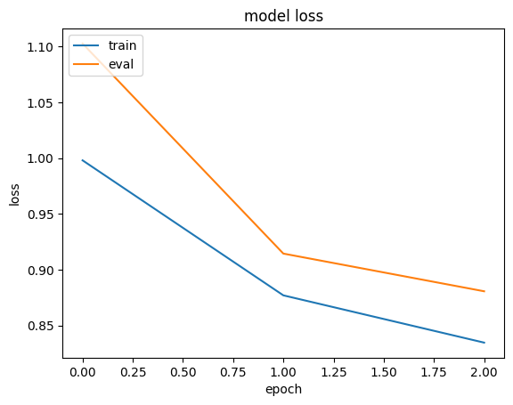
history = run_experiment(memory_efficient_model)

plt.plot(history.history["loss"])
plt.plot(history.history["val_loss"])
plt.title("model loss")
plt.ylabel("loss")
plt.xlabel("epoch")
plt.legend(["train", "eval"], loc="upper left")
plt.show()
Epoch 1/3
   6622/Unknown  6s 891us/step - loss: 1.1938 - mae: 0.8780

/Library/Frameworks/Python.framework/Versions/3.10/lib/python3.10/contextlib.py:153: UserWarning: Your input ran out of data; interrupting training. Make sure that your dataset or generator can generate at least `steps_per_epoch * epochs` batches. You may need to use the `.repeat()` function when building your dataset.
  self.gen.throw(typ, value, traceback)

 6646/6646 ━━━━━━━━━━━━━━━━━━━━ 7s 992us/step - loss: 1.1931 - mae: 0.8777 - val_loss: 1.1027 - val_mae: 0.8179
Epoch 2/3
 6646/6646 ━━━━━━━━━━━━━━━━━━━━ 7s 1ms/step - loss: 0.8908 - mae: 0.7488 - val_loss: 0.9144 - val_mae: 0.7549
Epoch 3/3
 6646/6646 ━━━━━━━━━━━━━━━━━━━━ 7s 980us/step - loss: 0.8419 - mae: 0.7278 - val_loss: 0.8806 - val_mae: 0.7419