知识蒸馏实践
作者:Sayak Paul
创建日期 2021/08/01
最后修改日期 2021/08/01
描述:通过函数匹配的知识蒸馏训练更好的学生模型。

简介
知识蒸馏(Hinton 等人)是一种使我们能够压缩大型模型为更小模型的技术。这使得我们能够获得高性能大型模型的优势,同时降低存储和内存成本,并提高推理速度。
- 更小的模型 -> 更小的内存占用
- 降低复杂度 -> 更少的浮点运算(FLOPs)
在《知识蒸馏:一个好老师是耐心且一致的》一文中,Beyer 等人研究了各种现有的知识蒸馏实现方法,并表明它们都导致了次优的性能。因此,在开发资源受限的生产系统时,实践者经常会选择其他替代方案(量化、剪枝、权重聚类等)。
Beyer 等人研究了如何改进知识蒸馏过程产生的学生模型,并使其性能始终与教师模型相匹配。在本示例中,我们将研究他们提出的实践方法,并使用 Flowers102 数据集。作为参考,作者使用这些实践方法,在 ImageNet-1k 数据集上取得了 82.8% 的准确率。
如果您需要回顾知识蒸馏的内容,并想学习如何在 Keras 中实现它,可以参考 此示例。您也可以参考 此示例,该示例展示了知识蒸馏在一致性训练中的扩展应用。
要运行此示例,您需要 TensorFlow 2.5 或更高版本以及 TensorFlow Addons,可以使用以下命令进行安装:
!pip install -q tensorflow-addons
导入
from tensorflow import keras
import tensorflow_addons as tfa
import tensorflow as tf

import matplotlib.pyplot as plt
import numpy as np

import tensorflow_datasets as tfds

tfds.disable_progress_bar()
超参数和常量
AUTO = tf.data.AUTOTUNE  # Used to dynamically adjust parallelism.
BATCH_SIZE = 64

# Comes from Table 4 and "Training setup" section.
TEMPERATURE = 10  # Used to soften the logits before they go to softmax.
INIT_LR = 0.003  # Initial learning rate that will be decayed over the training period.
WEIGHT_DECAY = 0.001  # Used for regularization.
CLIP_THRESHOLD = 1.0  # Used for clipping the gradients by L2-norm.

# We will first resize the training images to a bigger size and then we will take
# random crops of a lower size.
BIGGER = 160
RESIZE = 128
加载 Flowers102 数据集
train_ds, validation_ds, test_ds = tfds.load(
    "oxford_flowers102", split=["train", "validation", "test"], as_supervised=True
)
print(f"Number of training examples: {train_ds.cardinality()}.")
print(
    f"Number of validation examples: {validation_ds.cardinality()}."
)
print(f"Number of test examples: {test_ds.cardinality()}.")
Number of training examples: 1020.
Number of validation examples: 1020.
Number of test examples: 6149.
教师模型
与任何蒸馏技术一样,首先训练一个性能良好的教师模型非常重要,该模型通常比后续的学生模型要大。作者将一个 BiT ResNet152x2 模型(教师)蒸馏到一个 BiT ResNet50 模型(学生)中。
BiT 是 Big Transfer 的缩写,最早出现在 《Big Transfer (BiT): General Visual Representation Learning》 中。ResNets 的 BiT 变体使用组归一化(Wu 等人)和权重标准化(Qiao 等人)来替代批归一化(Ioffe 等人)。为了限制运行此示例所需的时间,我们将使用一个已在 Flowers102 数据集上训练好的 BiT ResNet101x3 模型。您可以参考 此 notebook 了解更多关于训练过程的信息。该模型在 Flowers102 的测试集上达到了 98.18% 的准确率。
模型权重托管在 Kaggle 的一个数据集中。要下载权重,请按照以下步骤操作:
- 在此 创建 Kaggle 账户。
- 转到您的 用户个人资料 的“账户”选项卡。
- 选择“创建 API Token”。这将触发下载
kaggle.json文件,其中包含您的 API 凭据。 - 从该 JSON 文件中复制您的 Kaggle 用户名和 API 密钥。
现在运行以下命令:
import os

os.environ["KAGGLE_USERNAME"] = "" # TODO: enter your Kaggle user name here
os.environ["KAGGLE_KEY"] = "" # TODO: enter your Kaggle key here
设置好环境变量后,运行:
$ kaggle datasets download -d spsayakpaul/bitresnet101x3flowers102
$ unzip -qq bitresnet101x3flowers102.zip
这应该会生成一个名为 T-r101x3-128 的文件夹,它本质上是一个教师 SavedModel。
import os

os.environ["KAGGLE_USERNAME"] = ""  # TODO: enter your Kaggle user name here
os.environ["KAGGLE_KEY"] = ""  # TODO: enter your Kaggle API key here
!kaggle datasets download -d spsayakpaul/bitresnet101x3flowers102
!unzip -qq bitresnet101x3flowers102.zip
# Since the teacher model is not going to be trained further we make
# it non-trainable.
teacher_model = keras.models.load_model(
    "/home/jupyter/keras-io/examples/keras_recipes/T-r101x3-128"
)
teacher_model.trainable = False
teacher_model.summary()
Model: "my_bi_t_model_1"
_________________________________________________________________
Layer (type)                 Output Shape              Param #
=================================================================
dense_1 (Dense)              multiple                  626790
_________________________________________________________________
keras_layer_1 (KerasLayer)   multiple                  381789888
=================================================================
Total params: 382,416,678
Trainable params: 0
Non-trainable params: 382,416,678
_________________________________________________________________
“函数匹配”实践
为了训练一个高质量的学生模型,作者提出了对学生训练工作流程进行以下更改:
- 使用 MixUp 的激进变体(Zhang 等人)。这是通过从均匀分布而不是 beta 分布中采样
alpha参数来实现的。MixUp 在这里用于帮助学生模型捕获教师模型所遵循的函数。MixUp 在数据流形上的不同样本之间进行线性插值。因此,这里的基本原理是,如果学生被训练来拟合,它应该能够更好地匹配教师模型。为了增加不变性,MixUp 与“Inception 风格”的裁剪(Szegedy 等人)结合使用。这就是“函数匹配”一词在 原始论文 中出现的原因。 - 与 Noisy Student Training 等其他作品不同,教师模型和学生模型接收图像的相同副本,该副本被混合并随机裁剪。通过向两个模型提供相同的输入,作者使得教师与学生保持一致。
- 使用 MixUp,我们在训练学生时实际上引入了一种强大的正则化形式。因此,它应该被训练相当长的时间(至少 1000 个 epoch)。由于学生是在强正则化下训练的,因此由于更长的训练计划而导致的过拟合风险也会得到缓解。
总而言之,在训练学生模型时需要保持一致和耐心。
数据输入管道
def mixup(images, labels):
    alpha = tf.random.uniform([], 0, 1)
    mixedup_images = alpha * images + (1 - alpha) * tf.reverse(images, axis=[0])
    # The labels do not matter here since they are NOT used during
    # training.
    return mixedup_images, labels


def preprocess_image(image, label, train=True):
    image = tf.cast(image, tf.float32) / 255.0

    if train:
        image = tf.image.resize(image, (BIGGER, BIGGER))
        image = tf.image.random_crop(image, (RESIZE, RESIZE, 3))
        image = tf.image.random_flip_left_right(image)
    else:
        # Central fraction amount is from here:
        # https://git.io/J8Kda.
        image = tf.image.central_crop(image, central_fraction=0.875)
        image = tf.image.resize(image, (RESIZE, RESIZE))

    return image, label


def prepare_dataset(dataset, train=True, batch_size=BATCH_SIZE):
    if train:
        dataset = dataset.map(preprocess_image, num_parallel_calls=AUTO)
        dataset = dataset.shuffle(BATCH_SIZE * 10)
    else:
        dataset = dataset.map(
            lambda x, y: (preprocess_image(x, y, train)), num_parallel_calls=AUTO
        )
    dataset = dataset.batch(batch_size)

    if train:
        dataset = dataset.map(mixup, num_parallel_calls=AUTO)

    dataset = dataset.prefetch(AUTO)
    return dataset
请注意,为了简洁起见,我们在训练集上使用了温和的裁剪,但在实践中应该应用“Inception 风格”的预处理。您可以参考 此脚本 以更详细地了解实现。此外,地面真实标签未用于训练学生模型。
train_ds = prepare_dataset(train_ds, True)
validation_ds = prepare_dataset(validation_ds, False)
test_ds = prepare_dataset(test_ds, False)
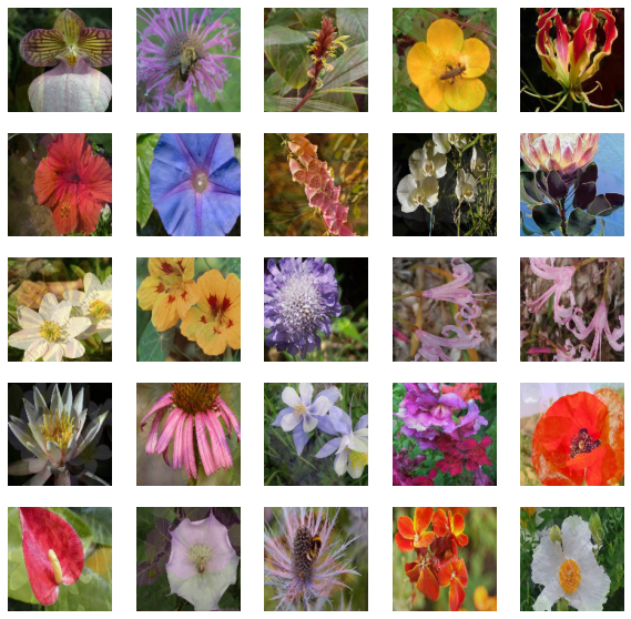
可视化
sample_images, _ = next(iter(train_ds))
plt.figure(figsize=(10, 10))
for n in range(25):
    ax = plt.subplot(5, 5, n + 1)
    plt.imshow(sample_images[n].numpy())
    plt.axis("off")
plt.show()
学生模型
在本示例中,我们将使用标准的 ResNet50V2(He 等人)。
def get_resnetv2():
    resnet_v2 = keras.applications.ResNet50V2(
        weights=None,
        input_shape=(RESIZE, RESIZE, 3),
        classes=102,
        classifier_activation="linear",
    )
    return resnet_v2


get_resnetv2().count_params()
23773798
与教师模型相比,该模型少了 3.58 亿个参数。
蒸馏实用程序
我们将重用 此有关知识蒸馏的示例 中的部分代码。
class Distiller(tf.keras.Model):
    def __init__(self, student, teacher):
        super().__init__()
        self.student = student
        self.teacher = teacher
        self.loss_tracker = keras.metrics.Mean(name="distillation_loss")

    @property
    def metrics(self):
        metrics = super().metrics
        metrics.append(self.loss_tracker)
        return metrics

    def compile(
        self, optimizer, metrics, distillation_loss_fn, temperature=TEMPERATURE,
    ):
        super().compile(optimizer=optimizer, metrics=metrics)
        self.distillation_loss_fn = distillation_loss_fn
        self.temperature = temperature

    def train_step(self, data):
        # Unpack data
        x, _ = data

        # Forward pass of teacher
        teacher_predictions = self.teacher(x, training=False)

        with tf.GradientTape() as tape:
            # Forward pass of student
            student_predictions = self.student(x, training=True)

            # Compute loss
            distillation_loss = self.distillation_loss_fn(
                tf.nn.softmax(teacher_predictions / self.temperature, axis=1),
                tf.nn.softmax(student_predictions / self.temperature, axis=1),
            )

        # Compute gradients
        trainable_vars = self.student.trainable_variables
        gradients = tape.gradient(distillation_loss, trainable_vars)

        # Update weights
        self.optimizer.apply_gradients(zip(gradients, trainable_vars))

        # Report progress
        self.loss_tracker.update_state(distillation_loss)
        return {"distillation_loss": self.loss_tracker.result()}

    def test_step(self, data):
        # Unpack data
        x, y = data

        # Forward passes
        teacher_predictions = self.teacher(x, training=False)
        student_predictions = self.student(x, training=False)

        # Calculate the loss
        distillation_loss = self.distillation_loss_fn(
            tf.nn.softmax(teacher_predictions / self.temperature, axis=1),
            tf.nn.softmax(student_predictions / self.temperature, axis=1),
        )

        # Report progress
        self.loss_tracker.update_state(distillation_loss)
        self.compiled_metrics.update_state(y, student_predictions)
        results = {m.name: m.result() for m in self.metrics}
        return results
学习率调度
论文中使用了预热余弦学习率调度。这种调度也是许多预训练方法的典型方法,尤其是在计算机视觉领域。
# Some code is taken from:
# https://www.kaggle.com/ashusma/training-rfcx-tensorflow-tpu-effnet-b2.


class WarmUpCosine(keras.optimizers.schedules.LearningRateSchedule):
    def __init__(
        self, learning_rate_base, total_steps, warmup_learning_rate, warmup_steps
    ):
        super().__init__()

        self.learning_rate_base = learning_rate_base
        self.total_steps = total_steps
        self.warmup_learning_rate = warmup_learning_rate
        self.warmup_steps = warmup_steps
        self.pi = tf.constant(np.pi)

    def __call__(self, step):
        if self.total_steps < self.warmup_steps:
            raise ValueError("Total_steps must be larger or equal to warmup_steps.")

        cos_annealed_lr = tf.cos(
            self.pi
            * (tf.cast(step, tf.float32) - self.warmup_steps)
            / float(self.total_steps - self.warmup_steps)
        )
        learning_rate = 0.5 * self.learning_rate_base * (1 + cos_annealed_lr)

        if self.warmup_steps > 0:
            if self.learning_rate_base < self.warmup_learning_rate:
                raise ValueError(
                    "Learning_rate_base must be larger or equal to "
                    "warmup_learning_rate."
                )
            slope = (
                self.learning_rate_base - self.warmup_learning_rate
            ) / self.warmup_steps
            warmup_rate = slope * tf.cast(step, tf.float32) + self.warmup_learning_rate
            learning_rate = tf.where(
                step < self.warmup_steps, warmup_rate, learning_rate
            )
        return tf.where(
            step > self.total_steps, 0.0, learning_rate, name="learning_rate"
        )
我们现在可以绘制使用此调度生成学习率的图表。
ARTIFICIAL_EPOCHS = 1000
ARTIFICIAL_BATCH_SIZE = 512
DATASET_NUM_TRAIN_EXAMPLES = 1020
TOTAL_STEPS = int(
    DATASET_NUM_TRAIN_EXAMPLES / ARTIFICIAL_BATCH_SIZE * ARTIFICIAL_EPOCHS
)
scheduled_lrs = WarmUpCosine(
    learning_rate_base=INIT_LR,
    total_steps=TOTAL_STEPS,
    warmup_learning_rate=0.0,
    warmup_steps=1500,
)

lrs = [scheduled_lrs(step) for step in range(TOTAL_STEPS)]
plt.plot(lrs)
plt.xlabel("Step", fontsize=14)
plt.ylabel("LR", fontsize=14)
plt.show()
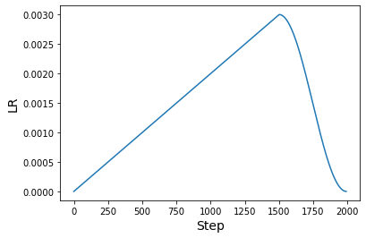
原始论文在进行“函数匹配”时使用了至少 1000 个 epoch 和 512 的批量大小。本示例的目的是展示实现该实践的方法,而不是展示全面应用时的结果。但是,这些实践方法将转移到论文中的原始设置。如果您有兴趣了解更多信息,请参考 此存储库。
训练
optimizer = tfa.optimizers.AdamW(
    weight_decay=WEIGHT_DECAY, learning_rate=scheduled_lrs, clipnorm=CLIP_THRESHOLD
)

student_model = get_resnetv2()

distiller = Distiller(student=student_model, teacher=teacher_model)
distiller.compile(
    optimizer,
    metrics=[keras.metrics.SparseCategoricalAccuracy()],
    distillation_loss_fn=keras.losses.KLDivergence(),
    temperature=TEMPERATURE,
)

history = distiller.fit(
    train_ds,
    steps_per_epoch=int(np.ceil(DATASET_NUM_TRAIN_EXAMPLES / BATCH_SIZE)),
    validation_data=validation_ds,
    epochs=30,  # This should be at least 1000.
)

student = distiller.student
student_model.compile(metrics=["accuracy"])
_, top1_accuracy = student.evaluate(test_ds)
print(f"Top-1 accuracy on the test set: {round(top1_accuracy * 100, 2)}%")
Epoch 1/30
16/16 [==============================] - 74s 3s/step - distillation_loss: 0.0070 - val_sparse_categorical_accuracy: 0.0039 - val_distillation_loss: 0.0061
Epoch 2/30
16/16 [==============================] - 37s 2s/step - distillation_loss: 0.0059 - val_sparse_categorical_accuracy: 0.0098 - val_distillation_loss: 0.0061
Epoch 3/30
16/16 [==============================] - 37s 2s/step - distillation_loss: 0.0049 - val_sparse_categorical_accuracy: 0.0098 - val_distillation_loss: 0.0060
Epoch 4/30
16/16 [==============================] - 37s 2s/step - distillation_loss: 0.0048 - val_sparse_categorical_accuracy: 0.0098 - val_distillation_loss: 0.0060
Epoch 5/30
16/16 [==============================] - 37s 2s/step - distillation_loss: 0.0043 - val_sparse_categorical_accuracy: 0.0098 - val_distillation_loss: 0.0060
Epoch 6/30
16/16 [==============================] - 37s 2s/step - distillation_loss: 0.0041 - val_sparse_categorical_accuracy: 0.0108 - val_distillation_loss: 0.0060
Epoch 7/30
16/16 [==============================] - 37s 2s/step - distillation_loss: 0.0038 - val_sparse_categorical_accuracy: 0.0098 - val_distillation_loss: 0.0061
Epoch 8/30
16/16 [==============================] - 37s 2s/step - distillation_loss: 0.0040 - val_sparse_categorical_accuracy: 0.0098 - val_distillation_loss: 0.0062
Epoch 9/30
16/16 [==============================] - 37s 2s/step - distillation_loss: 0.0039 - val_sparse_categorical_accuracy: 0.0098 - val_distillation_loss: 0.0063
Epoch 10/30
16/16 [==============================] - 37s 2s/step - distillation_loss: 0.0035 - val_sparse_categorical_accuracy: 0.0098 - val_distillation_loss: 0.0064
Epoch 11/30
16/16 [==============================] - 37s 2s/step - distillation_loss: 0.0041 - val_sparse_categorical_accuracy: 0.0098 - val_distillation_loss: 0.0064
Epoch 12/30
16/16 [==============================] - 37s 2s/step - distillation_loss: 0.0039 - val_sparse_categorical_accuracy: 0.0098 - val_distillation_loss: 0.0067
Epoch 13/30
16/16 [==============================] - 37s 2s/step - distillation_loss: 0.0039 - val_sparse_categorical_accuracy: 0.0098 - val_distillation_loss: 0.0067
Epoch 14/30
16/16 [==============================] - 37s 2s/step - distillation_loss: 0.0036 - val_sparse_categorical_accuracy: 0.0098 - val_distillation_loss: 0.0066
Epoch 15/30
16/16 [==============================] - 37s 2s/step - distillation_loss: 0.0037 - val_sparse_categorical_accuracy: 0.0098 - val_distillation_loss: 0.0065
Epoch 16/30
16/16 [==============================] - 37s 2s/step - distillation_loss: 0.0038 - val_sparse_categorical_accuracy: 0.0098 - val_distillation_loss: 0.0068
Epoch 17/30
16/16 [==============================] - 37s 2s/step - distillation_loss: 0.0039 - val_sparse_categorical_accuracy: 0.0098 - val_distillation_loss: 0.0066
Epoch 18/30
16/16 [==============================] - 37s 2s/step - distillation_loss: 0.0038 - val_sparse_categorical_accuracy: 0.0098 - val_distillation_loss: 0.0064
Epoch 19/30
16/16 [==============================] - 37s 2s/step - distillation_loss: 0.0035 - val_sparse_categorical_accuracy: 0.0098 - val_distillation_loss: 0.0071
Epoch 20/30
16/16 [==============================] - 37s 2s/step - distillation_loss: 0.0038 - val_sparse_categorical_accuracy: 0.0098 - val_distillation_loss: 0.0066
Epoch 21/30
16/16 [==============================] - 37s 2s/step - distillation_loss: 0.0038 - val_sparse_categorical_accuracy: 0.0098 - val_distillation_loss: 0.0068
Epoch 22/30
16/16 [==============================] - 37s 2s/step - distillation_loss: 0.0034 - val_sparse_categorical_accuracy: 0.0098 - val_distillation_loss: 0.0073
Epoch 23/30
16/16 [==============================] - 37s 2s/step - distillation_loss: 0.0035 - val_sparse_categorical_accuracy: 0.0098 - val_distillation_loss: 0.0078
Epoch 24/30
16/16 [==============================] - 37s 2s/step - distillation_loss: 0.0037 - val_sparse_categorical_accuracy: 0.0098 - val_distillation_loss: 0.0087
Epoch 25/30
16/16 [==============================] - 37s 2s/step - distillation_loss: 0.0031 - val_sparse_categorical_accuracy: 0.0108 - val_distillation_loss: 0.0078
Epoch 26/30
16/16 [==============================] - 37s 2s/step - distillation_loss: 0.0033 - val_sparse_categorical_accuracy: 0.0098 - val_distillation_loss: 0.0072
Epoch 27/30
16/16 [==============================] - 37s 2s/step - distillation_loss: 0.0036 - val_sparse_categorical_accuracy: 0.0098 - val_distillation_loss: 0.0071
Epoch 28/30
16/16 [==============================] - 37s 2s/step - distillation_loss: 0.0036 - val_sparse_categorical_accuracy: 0.0275 - val_distillation_loss: 0.0078
Epoch 29/30
16/16 [==============================] - 37s 2s/step - distillation_loss: 0.0032 - val_sparse_categorical_accuracy: 0.0196 - val_distillation_loss: 0.0068
Epoch 30/30
16/16 [==============================] - 37s 2s/step - distillation_loss: 0.0034 - val_sparse_categorical_accuracy: 0.0147 - val_distillation_loss: 0.0071
97/97 [==============================] - 7s 64ms/step - loss: 0.0000e+00 - accuracy: 0.0107
Top-1 accuracy on the test set: 1.07%
结果
仅进行 30 个 epoch 的训练,结果远未达到预期。这就是耐心(即更长的训练计划)的好处发挥作用的地方。让我们研究一下训练 1000 个 epoch 的模型能做什么。
# Download the pre-trained weights.
!wget https://git.io/JBO3Y -O S-r50x1-128-1000.tar.gz
!tar xf S-r50x1-128-1000.tar.gz
pretrained_student = keras.models.load_model("S-r50x1-128-1000")
pretrained_student.summary()
Model: "resnet"
_________________________________________________________________
Layer (type)                 Output Shape              Param #
=================================================================
root_block (Sequential)      (None, 32, 32, 64)        9408
_________________________________________________________________
block1 (Sequential)          (None, 32, 32, 256)       214912
_________________________________________________________________
block2 (Sequential)          (None, 16, 16, 512)       1218048
_________________________________________________________________
block3 (Sequential)          (None, 8, 8, 1024)        7095296
_________________________________________________________________
block4 (Sequential)          (None, 4, 4, 2048)        14958592
_________________________________________________________________
group_norm (GroupNormalizati multiple                  4096
_________________________________________________________________
re_lu_97 (ReLU)              multiple                  0
_________________________________________________________________
global_average_pooling2d_1 ( multiple                  0
_________________________________________________________________
head/dense (Dense)           multiple                  208998
=================================================================
Total params: 23,709,350
Trainable params: 23,709,350
Non-trainable params: 0
_________________________________________________________________
该模型完全遵循作者在学生模型中所使用的设置。这就是模型摘要略有不同的原因。
_, top1_accuracy = pretrained_student.evaluate(test_ds)
print(f"Top-1 accuracy on the test set: {round(top1_accuracy * 100, 2)}%")
97/97 [==============================] - 14s 131ms/step - loss: 0.0000e+00 - accuracy: 0.8102
Top-1 accuracy on the test set: 81.02%
经过 100000 个 epoch 的训练,同一模型实现了 95.54% 的 top-1 准确率。
论文中提供了许多重要的消融研究,这些研究表明与现有技术相比,这些实践方法的有效性。因此,如果您对此类方法持怀疑态度,请务必查阅论文。
关于延长训练时间的说明
借助基于 TPU 的硬件基础设施,我们可以更快地训练模型 1000 个 epoch。这甚至不需要对代码库进行大量更改。我们鼓励您查看 此存储库,因为它提供了适用于这些实践的 TPU 兼容训练工作流程,并且可以在 Kaggle Kernel 上运行,利用其免费的 TPU v3-8 硬件。