使用 node2vec 进行图表示学习
作者: Khalid Salama
创建日期 2021/05/15
最后修改日期 2021/05/15
描述:实现 node2vec 模型,为 MovieLens 数据集中的电影生成嵌入。

简介
从结构化为图的对象中学习有用的表示对于各种机器学习 (ML) 应用非常有用——例如社交和通信网络分析、生物医学研究和推荐系统。图表示学习旨在为图节点学习嵌入,这些嵌入可用于各种 ML 任务,例如节点标签预测(例如,根据文章的引用对其进行分类)和链接预测(例如,在社交网络中向用户推荐一个兴趣小组)。
node2vec 是一种简单但可扩展且有效的技术,通过优化保留邻域的目标来学习图中节点的低维嵌入。目标是根据图结构为相邻节点学习相似的嵌入。
给定结构化为图的数据项(其中项表示为节点,项之间的关系表示为边),node2vec 的工作原理如下:
- 使用(有偏的)随机游走生成项序列。
- 从这些序列创建正例和负例训练样本。
- 训练一个word2vec 模型(skip-gram)来学习项的嵌入。
在此示例中,我们在MovieLens 数据集的小版本上演示 node2vec 技术,以学习电影嵌入。这样的数据集可以通过将电影视为节点,并在具有相似用户评分的电影之间创建边来表示为一个图。学习到的电影嵌入可用于电影推荐或电影类型预测等任务。
此示例需要 networkx 包,可以使用以下命令安装:
pip install networkx
设置
import os
from collections import defaultdict
import math
import networkx as nx
import random
from tqdm import tqdm
from zipfile import ZipFile
from urllib.request import urlretrieve
import numpy as np
import pandas as pd
import tensorflow as tf
from tensorflow import keras
from tensorflow.keras import layers
import matplotlib.pyplot as plt
下载 MovieLens 数据集并准备数据
MovieLens 数据集的小版本包含来自 610 位用户对 9,742 部电影的大约 10 万条评分。
首先,我们下载数据集。下载的文件夹将包含三个数据文件:users.csv、movies.csv 和 ratings.csv。在此示例中,我们只需要 movies.dat 和 ratings.dat 数据文件。
urlretrieve(
    "http://files.grouplens.org/datasets/movielens/ml-latest-small.zip", "movielens.zip"
)
ZipFile("movielens.zip", "r").extractall()
然后,我们将数据加载到 Pandas DataFrame 中并进行一些基本预处理。
# Load movies to a DataFrame.
movies = pd.read_csv("ml-latest-small/movies.csv")
# Create a `movieId` string.
movies["movieId"] = movies["movieId"].apply(lambda x: f"movie_{x}")

# Load ratings to a DataFrame.
ratings = pd.read_csv("ml-latest-small/ratings.csv")
# Convert the `ratings` to floating point
ratings["rating"] = ratings["rating"].apply(lambda x: float(x))
# Create the `movie_id` string.
ratings["movieId"] = ratings["movieId"].apply(lambda x: f"movie_{x}")

print("Movies data shape:", movies.shape)
print("Ratings data shape:", ratings.shape)
Movies data shape: (9742, 3)
Ratings data shape: (100836, 4)
让我们检查一下 ratings DataFrame 的示例实例。
ratings.head()
| userId | movieId | rating | timestamp | |
|---|---|---|---|---|
| 0 | 1 | movie_1 | 4.0 | 964982703 |
| 1 | 1 | movie_3 | 4.0 | 964981247 |
| 2 | 1 | movie_6 | 4.0 | 964982224 |
| 3 | 1 | movie_47 | 5.0 | 964983815 |
| 4 | 1 | movie_50 | 5.0 | 964982931 |
接下来,让我们检查一下 movies DataFrame 的示例实例。
movies.head()
| movieId | title | genres | |
|---|---|---|---|
| 0 | movie_1 | Toy Story (1995) | Adventure|Animation|Children|Comedy|Fantasy |
| 1 | movie_2 | Jumanji (1995) | Adventure|Children|Fantasy |
| 2 | movie_3 | Grumpier Old Men (1995) | Comedy|Romance |
| 3 | movie_4 | Waiting to Exhale (1995) | Comedy|Drama|Romance |
| 4 | movie_5 | Father of the Bride Part II (1995) | Comedy |
为 movies DataFrame 实现两个实用函数。
def get_movie_title_by_id(movieId):
    return list(movies[movies.movieId == movieId].title)[0]


def get_movie_id_by_title(title):
    return list(movies[movies.title == title].movieId)[0]
构建电影图
如果两部电影由同一用户以 min_rating 或更高的评分进行评分,我们就为图中的两个电影节点创建一个边。边的权重将基于两部电影之间的点互信息,计算公式为:log(xy) - log(x) - log(y) + log(D),其中
xy是评分 ≥min_rating的用户中同时对电影x和电影y评分的数量。x是评分 ≥min_rating的用户中对电影x评分的数量。y是评分 ≥min_rating的用户中对电影y评分的数量。D是评分 ≥min_rating的电影评分总数。
步骤 1:创建电影之间的加权边。
min_rating = 5
pair_frequency = defaultdict(int)
item_frequency = defaultdict(int)

# Filter instances where rating is greater than or equal to min_rating.
rated_movies = ratings[ratings.rating >= min_rating]
# Group instances by user.
movies_grouped_by_users = list(rated_movies.groupby("userId"))
for group in tqdm(
    movies_grouped_by_users,
    position=0,
    leave=True,
    desc="Compute movie rating frequencies",
):
    # Get a list of movies rated by the user.
    current_movies = list(group[1]["movieId"])

    for i in range(len(current_movies)):
        item_frequency[current_movies[i]] += 1
        for j in range(i + 1, len(current_movies)):
            x = min(current_movies[i], current_movies[j])
            y = max(current_movies[i], current_movies[j])
            pair_frequency[(x, y)] += 1
Compute movie rating frequencies: 100%|███████████████████████████████████████████████████████████████████████████| 573/573 [00:00<00:00, 1049.83it/s]
步骤 2:使用节点和边创建图
为了减少节点之间的边数,只有当边的权重大于 min_weight 时,我们才添加边。
min_weight = 10
D = math.log(sum(item_frequency.values()))

# Create the movies undirected graph.
movies_graph = nx.Graph()
# Add weighted edges between movies.
# This automatically adds the movie nodes to the graph.
for pair in tqdm(
    pair_frequency, position=0, leave=True, desc="Creating the movie graph"
):
    x, y = pair
    xy_frequency = pair_frequency[pair]
    x_frequency = item_frequency[x]
    y_frequency = item_frequency[y]
    pmi = math.log(xy_frequency) - math.log(x_frequency) - math.log(y_frequency) + D
    weight = pmi * xy_frequency
    # Only include edges with weight >= min_weight.
    if weight >= min_weight:
        movies_graph.add_edge(x, y, weight=weight)
Creating the movie graph: 100%|███████████████████████████████████████████████████████████████████████████| 298586/298586 [00:00<00:00, 552893.62it/s]
让我们显示图中节点的总数和边的总数。请注意,节点数少于电影总数,因为只添加了有边连接到其他电影的电影。
print("Total number of graph nodes:", movies_graph.number_of_nodes())
print("Total number of graph edges:", movies_graph.number_of_edges())
Total number of graph nodes: 1405
Total number of graph edges: 40043
让我们显示图中节点的平均度(邻居数量)。
degrees = []
for node in movies_graph.nodes:
    degrees.append(movies_graph.degree[node])

print("Average node degree:", round(sum(degrees) / len(degrees), 2))
Average node degree: 57.0
步骤 3:创建词汇表并将 token 映射到整数索引
词汇表是图中的节点(电影 ID)。
vocabulary = ["NA"] + list(movies_graph.nodes)
vocabulary_lookup = {token: idx for idx, token in enumerate(vocabulary)}
实现有偏随机游走
随机游走从一个给定的节点开始,并随机选择一个邻居节点进行移动。如果边是加权的,则邻居是根据当前节点与其邻居之间的边的权重概率性地选择的。此过程重复 num_steps 次以生成一系列相关节点。
有偏随机游走通过引入以下两个参数来平衡广度优先采样(仅访问局部邻居)和深度优先采样(访问远距离邻居):
- 返回参数(
p):控制在游走中立即重新访问节点的可能性。将其设置为高值会鼓励适度探索,而将其设置为低值则会使游走保持局部。 - 入出参数(
q):允许搜索区分入向节点和出向节点。将其设置为高值会使随机游走偏向局部节点,而将其设置为低值会使游走偏向访问更远的节点。
def next_step(graph, previous, current, p, q):
    neighbors = list(graph.neighbors(current))

    weights = []
    # Adjust the weights of the edges to the neighbors with respect to p and q.
    for neighbor in neighbors:
        if neighbor == previous:
            # Control the probability to return to the previous node.
            weights.append(graph[current][neighbor]["weight"] / p)
        elif graph.has_edge(neighbor, previous):
            # The probability of visiting a local node.
            weights.append(graph[current][neighbor]["weight"])
        else:
            # Control the probability to move forward.
            weights.append(graph[current][neighbor]["weight"] / q)

    # Compute the probabilities of visiting each neighbor.
    weight_sum = sum(weights)
    probabilities = [weight / weight_sum for weight in weights]
    # Probabilistically select a neighbor to visit.
    next = np.random.choice(neighbors, size=1, p=probabilities)[0]
    return next


def random_walk(graph, num_walks, num_steps, p, q):
    walks = []
    nodes = list(graph.nodes())
    # Perform multiple iterations of the random walk.
    for walk_iteration in range(num_walks):
        random.shuffle(nodes)

        for node in tqdm(
            nodes,
            position=0,
            leave=True,
            desc=f"Random walks iteration {walk_iteration + 1} of {num_walks}",
        ):
            # Start the walk with a random node from the graph.
            walk = [node]
            # Randomly walk for num_steps.
            while len(walk) < num_steps:
                current = walk[-1]
                previous = walk[-2] if len(walk) > 1 else None
                # Compute the next node to visit.
                next = next_step(graph, previous, current, p, q)
                walk.append(next)
            # Replace node ids (movie ids) in the walk with token ids.
            walk = [vocabulary_lookup[token] for token in walk]
            # Add the walk to the generated sequence.
            walks.append(walk)

    return walks
使用有偏随机游走生成训练数据
您可以探索 p 和 q 的不同配置,以获得不同相关电影的结果。
# Random walk return parameter.
p = 1
# Random walk in-out parameter.
q = 1
# Number of iterations of random walks.
num_walks = 5
# Number of steps of each random walk.
num_steps = 10
walks = random_walk(movies_graph, num_walks, num_steps, p, q)

print("Number of walks generated:", len(walks))
Random walks iteration 1 of 5: 100%|█████████████████████████████████████████████████████████████████████████████| 1405/1405 [00:04<00:00, 291.76it/s]
Random walks iteration 2 of 5: 100%|█████████████████████████████████████████████████████████████████████████████| 1405/1405 [00:04<00:00, 302.56it/s]
Random walks iteration 3 of 5: 100%|█████████████████████████████████████████████████████████████████████████████| 1405/1405 [00:04<00:00, 294.52it/s]
Random walks iteration 4 of 5: 100%|█████████████████████████████████████████████████████████████████████████████| 1405/1405 [00:04<00:00, 304.06it/s]
Random walks iteration 5 of 5: 100%|█████████████████████████████████████████████████████████████████████████████| 1405/1405 [00:04<00:00, 302.15it/s]

Number of walks generated: 7025
生成正例和负例
为了训练 skip-gram 模型,我们使用生成的游走来创建正例和负例训练样本。每个样本包含以下特征:
target:游走序列中的一部电影。context:游走序列中的另一部电影。weight:这两部电影在游走序列中出现的次数。label:如果这两部电影是从游走序列中采样的,则标签为 1,否则(即,如果随机采样),则标签为 0。
生成示例
def generate_examples(sequences, window_size, num_negative_samples, vocabulary_size):
    example_weights = defaultdict(int)
    # Iterate over all sequences (walks).
    for sequence in tqdm(
        sequences,
        position=0,
        leave=True,
        desc=f"Generating positive and negative examples",
    ):
        # Generate positive and negative skip-gram pairs for a sequence (walk).
        pairs, labels = keras.preprocessing.sequence.skipgrams(
            sequence,
            vocabulary_size=vocabulary_size,
            window_size=window_size,
            negative_samples=num_negative_samples,
        )
        for idx in range(len(pairs)):
            pair = pairs[idx]
            label = labels[idx]
            target, context = min(pair[0], pair[1]), max(pair[0], pair[1])
            if target == context:
                continue
            entry = (target, context, label)
            example_weights[entry] += 1

    targets, contexts, labels, weights = [], [], [], []
    for entry in example_weights:
        weight = example_weights[entry]
        target, context, label = entry
        targets.append(target)
        contexts.append(context)
        labels.append(label)
        weights.append(weight)

    return np.array(targets), np.array(contexts), np.array(labels), np.array(weights)


num_negative_samples = 4
targets, contexts, labels, weights = generate_examples(
    sequences=walks,
    window_size=num_steps,
    num_negative_samples=num_negative_samples,
    vocabulary_size=len(vocabulary),
)
Generating positive and negative examples: 100%|██████████████████████████████████████████████████████████████████| 7025/7025 [00:11<00:00, 617.64it/s]
让我们显示输出的形状
print(f"Targets shape: {targets.shape}")
print(f"Contexts shape: {contexts.shape}")
print(f"Labels shape: {labels.shape}")
print(f"Weights shape: {weights.shape}")
Targets shape: (881412,)
Contexts shape: (881412,)
Labels shape: (881412,)
Weights shape: (881412,)
将数据转换为 tf.data.Dataset 对象
batch_size = 1024


def create_dataset(targets, contexts, labels, weights, batch_size):
    inputs = {
        "target": targets,
        "context": contexts,
    }
    dataset = tf.data.Dataset.from_tensor_slices((inputs, labels, weights))
    dataset = dataset.shuffle(buffer_size=batch_size * 2)
    dataset = dataset.batch(batch_size, drop_remainder=True)
    dataset = dataset.prefetch(tf.data.AUTOTUNE)
    return dataset


dataset = create_dataset(
    targets=targets,
    contexts=contexts,
    labels=labels,
    weights=weights,
    batch_size=batch_size,
)
训练 skip-gram 模型
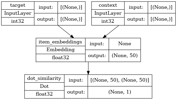
我们的 skip-gram 是一个简单的二元分类模型,其工作原理如下:
- 查找
target电影的嵌入。 - 查找
context电影的嵌入。 - 计算这两个嵌入之间的点积。
- 将结果(经过 sigmoid 激活后)与标签进行比较。
- 使用二元交叉熵损失。
learning_rate = 0.001
embedding_dim = 50
num_epochs = 10
实现模型
def create_model(vocabulary_size, embedding_dim):

    inputs = {
        "target": layers.Input(name="target", shape=(), dtype="int32"),
        "context": layers.Input(name="context", shape=(), dtype="int32"),
    }
    # Initialize item embeddings.
    embed_item = layers.Embedding(
        input_dim=vocabulary_size,
        output_dim=embedding_dim,
        embeddings_initializer="he_normal",
        embeddings_regularizer=keras.regularizers.l2(1e-6),
        name="item_embeddings",
    )
    # Lookup embeddings for target.
    target_embeddings = embed_item(inputs["target"])
    # Lookup embeddings for context.
    context_embeddings = embed_item(inputs["context"])
    # Compute dot similarity between target and context embeddings.
    logits = layers.Dot(axes=1, normalize=False, name="dot_similarity")(
        [target_embeddings, context_embeddings]
    )
    # Create the model.
    model = keras.Model(inputs=inputs, outputs=logits)
    return model
训练模型
我们实例化模型并进行编译。
model = create_model(len(vocabulary), embedding_dim)
model.compile(
    optimizer=keras.optimizers.Adam(learning_rate),
    loss=keras.losses.BinaryCrossentropy(from_logits=True),
)
让我们绘制模型。
keras.utils.plot_model(
    model,
    show_shapes=True,
    show_dtype=True,
    show_layer_names=True,
)
现在我们在 dataset 上训练模型。
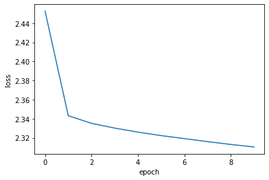
history = model.fit(dataset, epochs=num_epochs)
Epoch 1/10
860/860 [==============================] - 5s 5ms/step - loss: 2.4527
Epoch 2/10
860/860 [==============================] - 4s 5ms/step - loss: 2.3431
Epoch 3/10
860/860 [==============================] - 4s 4ms/step - loss: 2.3351
Epoch 4/10
860/860 [==============================] - 4s 4ms/step - loss: 2.3301
Epoch 5/10
860/860 [==============================] - 4s 5ms/step - loss: 2.3259
Epoch 6/10
860/860 [==============================] - 4s 4ms/step - loss: 2.3223
Epoch 7/10
860/860 [==============================] - 4s 5ms/step - loss: 2.3191
Epoch 8/10
860/860 [==============================] - 4s 4ms/step - loss: 2.3160
Epoch 9/10
860/860 [==============================] - 4s 4ms/step - loss: 2.3130
Epoch 10/10
860/860 [==============================] - 4s 5ms/step - loss: 2.3104
最后,我们绘制学习历史。
plt.plot(history.history["loss"])
plt.ylabel("loss")
plt.xlabel("epoch")
plt.show()
分析学习到的嵌入。
movie_embeddings = model.get_layer("item_embeddings").get_weights()[0]
print("Embeddings shape:", movie_embeddings.shape)
Embeddings shape: (1406, 50)
查找相关电影
定义一个包含一些电影的列表,称为 query_movies。
query_movies = [
    "Matrix, The (1999)",
    "Star Wars: Episode IV - A New Hope (1977)",
    "Lion King, The (1994)",
    "Terminator 2: Judgment Day (1991)",
    "Godfather, The (1972)",
]
获取 query_movies 中电影的嵌入。
query_embeddings = []

for movie_title in query_movies:
    movieId = get_movie_id_by_title(movie_title)
    token_id = vocabulary_lookup[movieId]
    movie_embedding = movie_embeddings[token_id]
    query_embeddings.append(movie_embedding)

query_embeddings = np.array(query_embeddings)
计算 query_movies 的嵌入与其他所有电影的嵌入之间的余弦相似度,然后为每部电影选取前 k 个。
similarities = tf.linalg.matmul(
    tf.math.l2_normalize(query_embeddings),
    tf.math.l2_normalize(movie_embeddings),
    transpose_b=True,
)

_, indices = tf.math.top_k(similarities, k=5)
indices = indices.numpy().tolist()
显示 query_movies 中最相关的电影。
for idx, title in enumerate(query_movies):
    print(title)
    print("".rjust(len(title), "-"))
    similar_tokens = indices[idx]
    for token in similar_tokens:
        similar_movieId = vocabulary[token]
        similar_title = get_movie_title_by_id(similar_movieId)
        print(f"- {similar_title}")
    print()
Matrix, The (1999)
------------------
- Matrix, The (1999)
- Raiders of the Lost Ark (Indiana Jones and the Raiders of the Lost Ark) (1981)
- Schindler's List (1993)
- Star Wars: Episode IV - A New Hope (1977)
- Lord of the Rings: The Fellowship of the Ring, The (2001)
Star Wars: Episode IV - A New Hope (1977)
-----------------------------------------
- Star Wars: Episode IV - A New Hope (1977)
- Schindler's List (1993)
- Raiders of the Lost Ark (Indiana Jones and the Raiders of the Lost Ark) (1981)
- Matrix, The (1999)
- Pulp Fiction (1994)
Lion King, The (1994)
---------------------
- Lion King, The (1994)
- Jurassic Park (1993)
- Independence Day (a.k.a. ID4) (1996)
- Beauty and the Beast (1991)
- Mrs. Doubtfire (1993)
Terminator 2: Judgment Day (1991)
---------------------------------
- Schindler's List (1993)
- Jurassic Park (1993)
- Terminator 2: Judgment Day (1991)
- Star Wars: Episode IV - A New Hope (1977)
- Back to the Future (1985)
Godfather, The (1972)
---------------------
- Apocalypse Now (1979)
- Fargo (1996)
- Godfather, The (1972)
- Schindler's List (1993)
- Casablanca (1942)
使用 Embedding Projector 可视化嵌入
import io

out_v = io.open("embeddings.tsv", "w", encoding="utf-8")
out_m = io.open("metadata.tsv", "w", encoding="utf-8")

for idx, movie_id in enumerate(vocabulary[1:]):
    movie_title = list(movies[movies.movieId == movie_id].title)[0]
    vector = movie_embeddings[idx]
    out_v.write("\t".join([str(x) for x in vector]) + "\n")
    out_m.write(movie_title + "\n")

out_v.close()
out_m.close()
下载 embeddings.tsv 和 metadata.tsv,以便在Embedding Projector 中分析获得的嵌入。
HuggingFace 上提供的示例
| 训练好的模型 | 演示 |
|---|---|